Natural Language Processing • Expectation Maximization
- Overview
- Expected Maximization
- Maximum Likelihood Estimation
- Gradient Descent
- The difference between them all
Overview
- In this article, we will discuss the nuanced differences between Expected Maximization, MLE, and Gradient Descent.
Expected Maximization
- The Expectation-Maximization (EM) algorithm is an iterative approach used to estimate the parameters in statistical models that involve unobserved latent variables. It aims to find the maximum likelihood or maximum a posteriori estimates of these parameters.
- The EM iteration consists of two steps: the Expectation (E) step and the Maximization (M) step. In the E step, the algorithm computes the expectation of the log-likelihood using the current parameter estimates. This step involves creating a function that represents the expected log-likelihood. The M step follows, where the algorithm maximizes this expected log-likelihood to compute updated parameter estimates.
- The EM algorithm repeats these steps iteratively, with each iteration providing improved parameter estimates. The estimated parameters are then used to determine the distribution of the latent variables in the next E step. By alternating between the E and M steps, the EM algorithm iteratively refines the parameter estimates until convergence is reached.
- The EM algorithm is a powerful iterative method for estimating model parameters in statistical models with unobserved latent variables. It combines the E step to calculate the expectation of the log-likelihood and the M step to maximize the expected log-likelihood, ultimately refining the parameter estimates throughout the iterations.
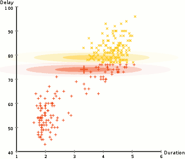
- The image below (source), does a great job at representing that.
- This is an algorithm for parameter estimation in statistical models where the model depends on unobserved latent variables. EM alternates between performing an expectation (E) step, which creates a function for the expectation of the log-likelihood evaluated using the current estimate for the parameters, and a maximization (M) step, which computes parameters maximizing the expected log-likelihood found on the E step.
- In a sense, EM is an algorithm that encompasses both MLE (as it’s used to maximize the likelihood) and optimization (as it iteratively maximizes a function).
- It is another method for parameter estimation, used when the model includes latent (hidden) variables. It’s a more complex method than MLE, and it’s also an iterative algorithm. It alternates between an Expectation step (which computes a probability distribution over possible values of the latent variables given the current parameters) and a Maximization step (which updates the parameters based on this distribution).
- In NLP, the EM algorithm is frequently used when dealing with models that involve latent or hidden variables. For instance, in the task of topic modeling (where the goal is to discover the main topics that occur in a document collection), one popular method is Latent Dirichlet Allocation (LDA). LDA assumes that each document is a mixture of a small number of topics, and that each word in the document is attributable to one of the document’s topics. However, the topics themselves are not observed (they’re latent variables), and we use the EM algorithm to estimate both the topic distribution for each document and the word distribution for each topic.
- The Expectation-Maximization algorithm is used when the model depends on unobserved latent variables. It is an iterative method that starts with a guess about the parameters and improves it iteratively.
- The algorithm consists of two steps:
- Expectation step (E-step): Given the current estimate of the parameters, the expectation of the log-likelihood is computed.
- Maximization step (M-step): Parameters are updated such that the expectation of the log-likelihood found in the E-step is maximized.
- The algorithm consists of two steps:
- Pros:
- Efficiently deals with models with hidden or latent variables, where MLE is not applicable.
- Can work with missing data.
- Generally converges to a local maximum of the likelihood function.
- Cons:
- It’s an iterative method, so it may be slower than direct methods like MLE.
- The algorithm may converge to a local maximum rather than the global maximum of the likelihood function.
- The initialization of parameters can significantly affect the final solution.
Maximum Likelihood Estimation
- MLE is a method of estimating the parameters of a statistical model given observations. MLE attempts to find the parameter values that maximize the likelihood function, given the data. In other words, MLE finds the parameter values that make the observed data most probable.
- MLE is a type of parameter estimation, but it’s not an optimization algorithm per se. Instead, it’s a principle or method on which an optimization problem can be based.
- This is a method of estimating the parameters of a statistical model given observations. MLE attempts to find the parameter values that maximize the likelihood function, given the data. In other words, MLE finds the parameter values that make the observed data most probable. MLE is a type of parameter estimation, but it’s not an optimization algorithm per se. Instead, it’s a principle or method on which an optimization problem can be based.
- It is a specific approach to parameter estimation in probabilistic models. Given a set of data and a model, MLE finds the parameters that make the observed data most probable under the model. If we define a loss function that is the negative log-likelihood of the data, then MLE becomes an optimization problem that can be solved with gradient descent (or other optimization algorithms).
- In the context of NLP, MLE is commonly used in language modeling. For instance, in the n-gram language model, we estimate the probabilities of sequences of words appearing in the language based on observed frequencies in the training data.
- We choose the model parameters (these probabilities) that maximize the likelihood of our observed data. This is done through MLE. Here’s an oversimplified example: given a corpus, we might want to find the probability of the word ‘apple’ following the word ‘red’. We would count the number of times ‘red apple’ occurs and divide it by the number of times ‘red’ occurs to get the MLE estimate.
- So you would use MLE when you can compute the likelihood directly and your model doesn’t contain hidden or latent variables. On the other hand, you would use EM when dealing with latent variables or missing data, where the likelihood is difficult to compute directly.
- Maximum Likelihood Estimation is a method of estimating the parameters of a statistical model. Given an observed dataset, the MLE technique aims to find the parameters that maximize the likelihood function. These parameters will be the best representation of the data according to the model.
- Pros:
- Straightforward and simple to implement.
- Asymptotically unbiased, meaning that as the size of the sample data increases, the MLEs converge to the true parameter values.
- Provides a single point estimate of model parameters.
- Cons:
- Might be difficult to solve analytically for complex models.
- Can overfit the data if not regularized properly.
- Doesn’t work well with models that have hidden or latent variables, as it’s hard to calculate the likelihood directly in these cases.
Gradient Descent
- This is an optimization algorithm used to find the values of parameters (coefficients) of a function (f) that minimizes a cost function (cost).
- Gradient descent is best used when the parameters cannot be calculated analytically (e.g., using linear algebra) and must be searched for iteratively.
- It is a general-purpose optimization algorithm that can be used to find the parameters that minimize (or maximize) any differentiable function.
- In machine learning, it’s often used to minimize the loss function, which measures the difference between the model’s predictions and the actual data. The algorithm iteratively adjusts the parameters in the direction that reduces the loss the most, until it hopefully arrives at a minimum.
The difference between them all
- In a typical machine learning task, MLE or EM might be used to formulate the optimization problem (i.e., to define what it means for one set of parameters to be better than another), and then an optimization algorithm like Gradient Descent might be used to solve this problem (i.e., to find the best set of parameters according to the criterion defined by MLE or EM).
- While all three methods can be used for optimization, Gradient Descent is a general optimization algorithm, while MLE and EM are specific methods for parameter estimation in probabilistic models. Gradient Descent can actually be used as part of the solution method in MLE or EM, when we need to solve an optimization problem to update the parameters.
|                     | Gradient Descent                 | Maximum Likelihood Estimation (MLE) | Expectation Maximization (EM)              |
|---------------------|----------------------------------|-------------------------------------|-------------------------------------------|
| Basic Concept       | An optimization algorithm that iteratively adjusts parameters to minimize a cost function. | A statistical method for estimating the parameters of a model that maximizes the likelihood of the observed data. | A statistical method to find maximum likelihood or MAP estimates for models with latent variables or incomplete data. |
| Use Cases           | Useful when the cost function is differentiable. Widely used in training various types of machine learning models. | Used when we have a parametric model of the data and we want to find the parameters that best explain the observed data. | Used when there are hidden or latent variables in the model or when data is missing or incomplete. |
| Operation           | Works by iteratively updating parameters in the direction of the negative gradient. | Maximizes the likelihood function to find the best parameters. | Alternates between an expectation (E) step and a maximization (M) step. |
| Strengths           | Can be used for a wide range of problems. Easy to implement. | Provides a principled way of deriving estimators. | Can handle hidden variables and incomplete data. |
| Limitations         | Requires the function to be differentiable. Can get stuck in local minima for non-convex functions. | Can be computationally challenging for complex models. Does not handle hidden variables directly. | Can be computationally expensive. Convergence to local maximum is guaranteed, but not to the global maximum. |