NLP • Neural Architectures
- Overview
- Recurrent Neural Networks (RNN)
- Gated Recurrent Units (GRU)
- Convolutional Neural Networks (CNN)
- Transformer Models
- BERT, GPT, and Other Variants
- Multilayer Perceptron
- ResNets
- How does ResNet-50 solve the vanishing gradients problem of VGG-16?
- Seq2Seq Architecture in NLP
Overview
- The goal of NLP is to read, decipher, understand, and make sense of human language in a valuable way.
- To achieve this, various machine learning models have been developed and utilized, each with its unique architecture and use-cases.
- Let’s explore some prevalent neural architectures used in NLP.
Recurrent Neural Networks (RNN)
- Recurrent Neural Networks, or RNNs, are a type of artificial neural network designed to recognize patterns in sequences of data, such as text, genomes, handwriting, or spoken words. A key feature of RNNs is their “memory”. Output from previous steps are fed into subsequent steps, allowing information to persist through the network, which can be particularly useful when dealing with sequences of words.
- However, RNNs can suffer from problems like vanishing gradients, making them hard to train over long sequences. They also process data sequentially, which can be a disadvantage when dealing with large datasets because it’s difficult to parallelize the computations.
- The image below (source) displays RNNs architecture.
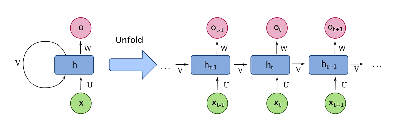
- A recurrent neural network (RNN) is a type of artificial neural network that allows connections between nodes to form cycles, enabling the output from certain nodes to influence subsequent inputs to those same nodes. This characteristic empowers RNNs to exhibit temporal dynamics, distinguishing them from traditional feedforward neural networks. By utilizing an internal state or memory, RNNs are capable of processing sequences of inputs with varying lengths. This feature makes them suitable for tasks like unsegmented, connected handwriting recognition or speech recognition. Notably, recurrent neural networks possess the property of Turing completeness, enabling them to execute arbitrary programs for processing diverse sequences of inputs.
- The term “recurrent neural network” specifically refers to networks with an infinite impulse response, whereas “convolutional neural network” pertains to networks with a finite impulse response. Both types of networks display temporal dynamic behavior. A finite impulse recurrent network can be represented as a directed acyclic graph that can be unfolded and replaced with a strictly feedforward neural network. On the other hand, an infinite impulse recurrent network takes the form of a directed cyclic graph that cannot be unfolded.
- Both finite impulse and infinite impulse recurrent networks can incorporate additional stored states, which can be directly controlled by the neural network. These storage elements can also be substituted with another network or graph that incorporates time delays or feedback loops. These controlled states are often referred to as gated states or gated memory and play a role in long short-term memory networks (LSTMs) and gated recurrent units. This architecture is sometimes known as a Feedback Neural Network (FNN).
- Recurrent Neural Networks (RNN) are a type of artificial neural network that’s well-suited for processing sequential data. Unlike feedforward neural networks, which process inputs independently, RNNs possess a form of internal memory that allows them to take into account previous inputs in the sequence when producing the current output.
How Does an RNN Work Internally?
- The key to an RNN’s design is a hidden state, which acts as the network’s memory. For each element in a sequence, the RNN performs a computation that includes both the current input and the previously computed hidden state. The result of this computation becomes the new hidden state, which gets passed on to the next step.
- Mathematically, this can be described as:
hidden_state_t = f(U*input_t + W*hidden_state_t-1)
- Where:
input_tis the current inputhidden_state_tis the current hidden statehidden_state_t-1is the previous hidden stateUandWare weight matrices-
fis an activation function, such as tanh or ReLU - This structure forms a loop, or recurrence, that allows information to be carried across steps in the sequence.
What Tasks are RNNs Used for in NLP?
- Given their ability to process sequential data, RNNs are commonly used in many NLP tasks, including:
- Sentiment Analysis: RNNs can analyze sequences of words to determine the sentiment expressed in text, such as identifying whether a product review is positive or negative.
- Text Generation: RNNs can generate human-like text by predicting the next word in a sequence given the previous words.
- Machine Translation: RNNs can be used in systems that translate text from one language to another.
- Speech Recognition: RNNs can transcribe spoken language into written text.
Benefits of RNNs
- Ability to Handle Sequences: RNNs are designed to effectively handle sequential data, making them particularly well-suited for NLP tasks.
- Memory of Past Information: The hidden state acts as a form of memory, allowing an RNN to take into account prior context when making a decision.
Cons of RNNs
- Vanishing Gradient Problem: During training, RNNs can suffer from the vanishing gradient problem, where the contributions of information decay geometrically over time, making it difficult for the RNN to learn long-range dependencies.
- Difficulty with Long Sequences: Related to the vanishing gradient problem, RNNs can struggle with long sequences, as the information from early steps in the sequence can be diluted by the time it reaches the end.
- Computational Intensity: Because of their sequential nature, RNNs can be slow to train, as it’s difficult to parallelize the computations.
- To address some of these issues, variants of RNNs like Long Short-Term Memory units (LSTM) and Gated Recurrent units (GRU) were developed. They introduce concepts of gating and memory cells that can control the flow of information and effectively capture long-term dependencies in the data.
Long Short-Term Memory (LSTM)
- LSTMs are a special kind of RNN, capable of learning long-term dependencies, which makes them exceptionally well-suited for many NLP tasks. They work on the principle of selectively remembering patterns over a duration of time.
- Unlike traditional RNNs, LSTMs use a series of “gates” to control the flow of information into and out of the memory, mitigating the vanishing gradient problem and allowing the model to learn from data where relevant events are separated by large gaps.
- Long Short-Term Memory (LSTM) networks are a type of recurrent neural network (RNN) designed to learn from experience to classify, process, and predict time series when there are very long time lags of unknown size between important events. As a special kind of RNN, LSTMs are particularly well-suited for many NLP tasks.
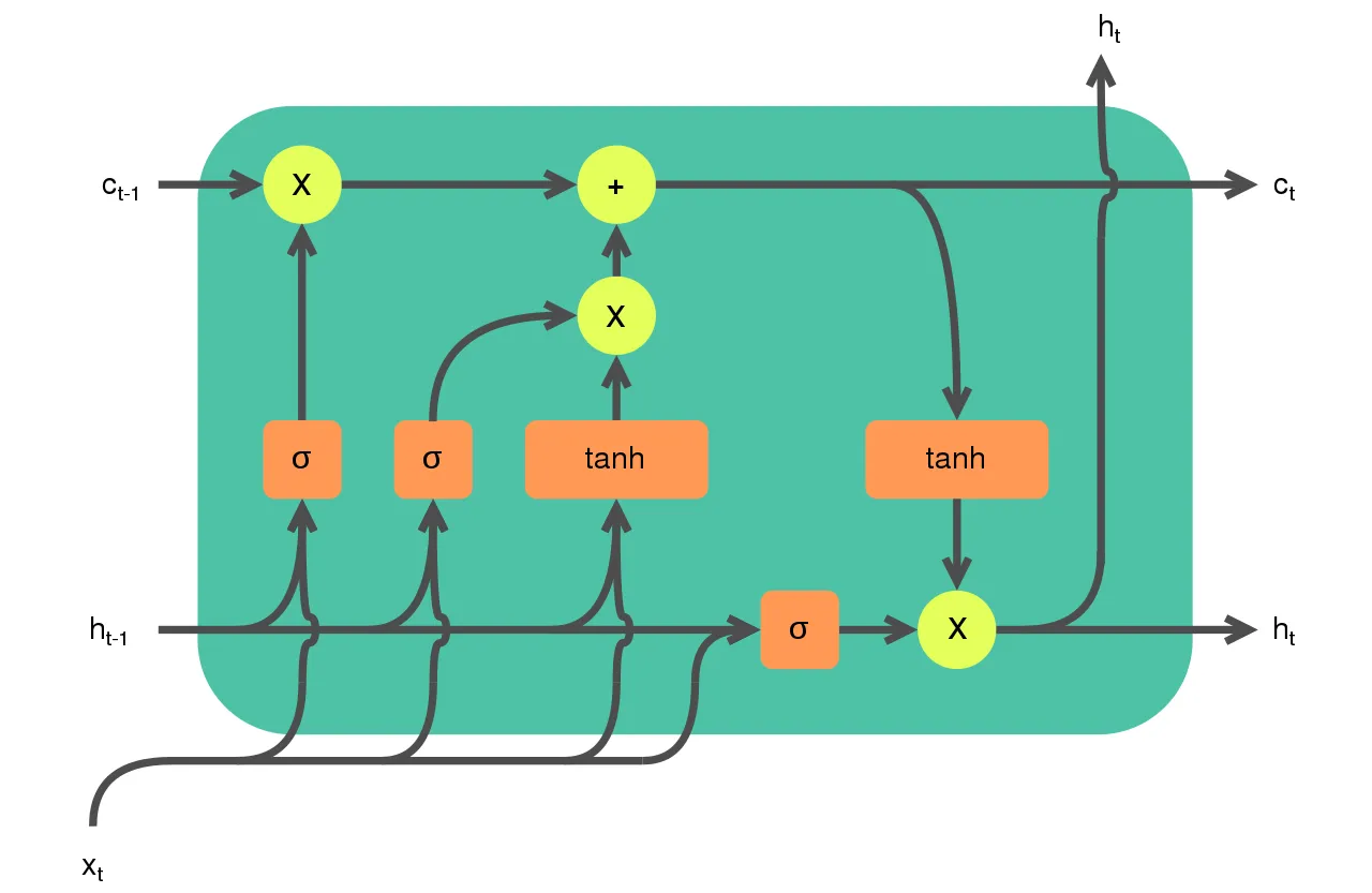
- The image below (source), displays the gates of LSTMs.
How Does an LSTM Work Internally?
- The secret sauce of LSTMs is their ability to remember and recall information for an extended period. This capability is facilitated by a complex system of “gates”. An LSTM unit includes an input gate, forget gate, and output gate, each playing a specific role:
- Input Gate: Decides how much of the incoming information to store in the cell state.
- Forget Gate: Determines how much of the existing cell state to retain.
- Output Gate: Decides what information from the current cell state to output.
- Mathematically, these operations are represented as:
forget_gate = sigmoid(W_f*[h_t-1, x_t] + b_f)
input_gate = sigmoid(W_i*[h_t-1, x_t] + b_i)
output_gate = sigmoid(W_o*[h_t-1, x_t] + b_o)
new_memory_cell = tanh(W_c*[h_t-1, x_t] + b_c)
cell_state_t = forget_gate*cell_state_t-1 + input_gate*new_memory_cell
hidden_state_t = output_gate*tanh(cell_state_t)
- Where:
h_t-1is the previous hidden statex_tis the current inputcell_state_tis the current cell stateWandbare weight matrices and bias vectorssigmoidandtanhare activation functions
What Tasks are LSTMs Used for in NLP?
- LSTMs are well-suited for classifying, processing, and making predictions based on time series data, which makes them exceptionally useful for many NLP tasks, including:
- Machine Translation: LSTMs can be used in sequence-to-sequence prediction problems, such as translating English text to French text.
- Text Generation: LSTM’s ability to remember long sequences makes it excellent for generating sentences or even whole paragraphs of text.
- Speech Recognition: LSTMs are used in transcription services to convert spoken language into written form.
- Sentiment Analysis: LSTMs can analyze context over longer sequences, making them effective at understanding the sentiment expressed in sentences or even whole documents.
Benefits of LSTMs
- Long-Range Dependencies: LSTMs can capture long-term dependencies and patterns in sequence data due to the gating mechanism, which is not possible with traditional RNNs.
- Avoiding the Vanishing Gradient Problem: LSTMs tackle the vanishing gradient problem effectively, allowing them to learn from data where relevant events are separated by large time lags.
Cons of LSTMs
- Computational Complexity: Due to the complex gating mechanism, LSTMs require more computational resources and can be slower to train compared to simpler models like the basic RNN or GRU.
- Requires Large Datasets: To realize their full potential, LSTMs typically require large amounts of data and may not be suitable for tasks with limited data.
- Overfitting: Without careful design and regularization, LSTM models might overfit to the training data, especially when the dataset is small.
- By addressing the shortcomings of basic RNNs and providing a way to capture long-term dependencies in sequence data, LSTMs represent a major advancement in the field of NLP and continue to be a key tool in many state-of-the-art systems.
Gated Recurrent Units (GRU)
- The GRU is the newer generation of Recurrent Neural networks and is pretty similar to an LSTM. GRUs, however, combine the forget and input gates into a single “update gate”. They also merge the cell state and hidden state, resulting in a simpler model. While this can make GRUs computationally more efficient than LSTMs, the choice between GRU and LSTM usually depends on the specific requirements of a task and the data available.
- Gated Recurrent Units (GRU) is a type of recurrent neural network introduced by Kyunghyun Cho in 2014. They are similar to the more widely known Long Short-Term Memory (LSTM) units but are somewhat simpler and thus computationally more efficient.
How Does a GRU Work Internally?
- A GRU has two gates (update and reset) and two states (hidden state and new memory), compared to the LSTM’s three gates and two states. Here’s a breakdown of each component:
- Update Gate: Determines how much of the previous hidden state to keep around. If the update gate is close to 1, the previous hidden state is mostly passed along to the next time step.
- Reset Gate: Determines how much of the previous hidden state to forget.
-
The main difference compared to LSTM is that in a GRU, the hidden state and cell state are combined into a single hidden state. The GRU’s hidden state can directly feed into the next layer of a neural network, which can make it more efficient.
- Mathematically, these operations are represented as:
update_gate = sigmoid(W_u*[h_t-1, x_t] + b_u)
reset_gate = sigmoid(W_r*[h_t-1, x_t] + b_r)
new_memory = tanh(W*[reset_gate*h_t-1, x_t] + b)
hidden_state_t = (1 - update_gate)*new_memory + update_gate*h_t-1
- Where:
h_t-1is the previous hidden statex_tis the current inputWandbare weight matrices and bias vectorssigmoidandtanhare activation functions
What Tasks are GRUs Used for in NLP?
- Like LSTMs, GRUs are used for a range of NLP tasks, including:
- Machine Translation: GRUs can translate text from one language to another by understanding the context of each word in a sentence.
- Sentiment Analysis: GRUs can analyze sequences of words to determine the sentiment expressed in the text.
- Text Generation: GRUs can generate human-like text by predicting the next word in a sequence given the previous words.
- Named Entity Recognition: GRUs can classify words in a sentence into pre-defined categories like person names, organizations, locations, medical codes, time expressions, quantities, monetary values, percentages, etc.
Benefits of GRUs
- Efficiency: The GRU’s simpler structure means it’s easier to modify and computationally more efficient than the LSTM. It uses fewer resources and trains faster.
- Performance: Despite its simplicity, the GRU can perform as well as the LSTM on many tasks and is sometimes the preferred choice when computational resources are limited.
Cons of GRUs
- Lack of Flexibility: The GRU’s simpler design makes it less flexible than the LSTM, which may limit its performance on certain tasks.
- Requires Large Datasets: Like LSTMs, GRUs typically require large amounts of data to realize their full potential and may not be suitable for tasks with limited data.
- In conclusion, while GRUs are simpler and faster to compute than LSTMs, the choice between the two often depends on the specific requirements of the task and the computational resources available. It’s often worth trying both to see which performs better on a given task.
Convolutional Neural Networks (CNN)
- While CNNs are usually associated with image processing, they’ve also proven useful for NLP tasks. CNNs use a technique called convolution to focus on local regions of the input, identifying patterns in each region. This architecture can be used to identify local word patterns or n-grams in a sentence, providing a more global understanding of the text.
- Convolutional Neural Networks (CNN) are a class of deep learning models primarily used for processing grid-like data such as images. However, their ability to identify local and shift-invariant features also makes them well-suited for certain Natural Language Processing (NLP) tasks.
How Does a CNN Work Internally?
- In an NLP context, a sentence is often treated as a 1D sequence, with each word or character represented as a multi-dimensional vector (a point in high-dimensional space). The fundamental operation in a CNN is the convolution, which involves a filter (also called a kernel) that scans across the sequence and produces a new sequence that represents the presence of certain features.
- These features could be as simple as the presence of a certain word or as complex as a particular sequence of words with specific semantic or syntactic properties. By stacking multiple convolutional layers with non-linear activation functions, a CNN can learn to identify complex features in the input data.
- Max-pooling is another common operation in CNNs, which reduces the dimensionality of the data while preserving the most salient features. This operation helps make the model more efficient and less prone to overfitting.
What Tasks are CNNs Used for in NLP?
- Text Classification: CNNs are highly effective at text classification tasks, such as sentiment analysis or topic categorization, where local features, like certain sequences of words or phrases, are highly predictive of the class.
- Named Entity Recognition: CNNs can identify named entities in text, such as names of people, organizations, locations, expressions of times, quantities, percentages, etc.
- Sentence Modeling: CNNs can be used to encode sentences in a dense vector space, where semantically similar sentences are close together.
Benefits of CNNs
- Efficiency: CNNs tend to be more computationally efficient than RNNs for certain tasks, particularly on tasks with fixed-length inputs.
- Capture Local Features: CNNs are excellent at identifying local and shift-invariant features. In the context of NLP, this means they can detect meaningful phrases or combinations of words irrespective of their position in the sentence.
Cons of CNNs
- Limited Contextual Understanding: Unlike RNNs or Transformers, CNNs have a fixed-size receptive field (determined by the kernel size), which means they cannot natively incorporate context from words farther away. While this can be mitigated to some extent with larger kernel sizes and multiple layers, CNNs fundamentally have a more limited contextual understanding compared to some other model architectures.
- Struggle with Long Sequences: CNNs can struggle to handle long sequences effectively, especially when important features are dispersed across the sequence.
- In summary, while CNNs might not be the first choice for many NLP tasks in the era of Transformers, they can still be an effective tool in the NLP toolkit, particularly for tasks involving classification or where the identification of local features is important.
Transformer Models
- Transformer models, introduced in the paper “Attention is All You Need” by Vaswani et al., brought a revolution in NLP. They rely entirely on a mechanism called self-attention, forgoing recurrence and convolutions.
- Transformers handle ordering by injecting position-specific information into the input and can process all elements of a sequence in parallel, making them much more scalable than RNNs or LSTMs.
- The Transformer is a type of deep learning model introduced in 2017 in the paper “Attention is All You Need” by Vaswani et al. It marked a departure from the recurrent style of models like LSTMs and GRUs, instead using a self-attention mechanism to process data. Transformers have proven to be highly effective and are at the heart of many state-of-the-art models in NLP, including BERT, GPT-3, and T5.
How Does a Transformer Work Internally?
- A Transformer consists of an encoder and a decoder. Each of them is composed of a stack of identical layers. The layers in the encoder process the input data simultaneously rather than sequentially, which makes them highly parallelizable.
- The key innovation in the Transformer model is the self-attention mechanism, also known as scaled dot-product attention. This allows the model to weigh the importance of different words in a sentence when generating an encoding for a particular word.
- In more technical terms, for each word, the transformer generates a Query, a Key, and a Value (Q, K, and V). These are vectors that are computed from the word’s embedding. The attention score for a given word is then calculated as the dot product of the Query with all Keys, followed by a softmax operation.
- The final output of the attention layer for each word is a weighted sum of all Values, where the weights are the attention scores. This process allows the model to focus on different words to varying degrees when encoding each word.
What Tasks are Transformers Used for in NLP?
- Transformers have been successful across a wide range of NLP tasks:
- Machine Translation: Transformers have achieved state-of-the-art performance on tasks like translating English text to German and French.
- Text Summarization: Transformers can condense a long document into a short summary while maintaining the main points of the original text.
- Question Answering: Transformers can understand a passage of text and answer questions about its content.
- Sentiment Analysis: Transformers can classify text as expressing positive, negative, or neutral sentiment.
- Text Generation: Transformers can generate human-like text given some initial prompt.
Benefits of Transformers
- Parallelization: Unlike RNNs and their variants, Transformers don’t require sequential data processing, making them much more efficient on modern hardware, which is designed for parallel operations.
- Long-Range Dependencies: The self-attention mechanism allows Transformers to handle long-range dependencies in text more effectively than RNNs.
- Versatility: Transformers have proven to be highly effective on a wide range of NLP tasks, and are the backbone of many state-of-the-art NLP models.
Cons of Transformers
- Resource Intensive: Transformers can require significant computational resources and memory, particularly for longer sequences. This is due in part to the self-attention mechanism, which is quadratic in the sequence length.
- Overfitting: Like other deep learning models, Transformers can overfit to the training data, especially when the dataset is small.
- Transformers have revolutionized the field of NLP and are likely to remain at the forefront of research in the coming years. Their success has also spurred interest in developing more efficient and powerful variants, such as the Transformer-XL and the Reformer.
BERT, GPT, and Other Variants
- Building on the Transformer architecture, models like BERT (Bidirectional Encoder Representations from Transformers) and GPT (Generative Pretrained Transformer) have significantly improved performance on a wide range of NLP tasks.
- BERT uses the Transformer’s encoder mechanism in a bidirectional manner to understand the context of each word in relation to all its surrounding words. On the other hand, GPT uses the Transformer’s decoder mechanism and learns to predict the next word in a sequence, gaining a comprehensive understanding of language syntax and semantics.
- The choice of architecture often depends on the specific requirements of the task at hand, including the amount of data available, the complexity of the task, and the computational resources at one’s disposal. However, as the field continues to evolve, we can look forward to even more sophisticated models that push the boundaries of what’s possible in NLP.
- BERT, introduced by Google in 2018, is a Transformer-based model that stands for Bidirectional Encoder Representations from Transformers. It is designed to pre-train deep bidirectional representations from unlabeled text by jointly conditioning on both left and right context. This allows the model to learn the context of a word based on all of its surroundings (left and right of the word).
- Unlike previous models, BERT is designed to pre-train deep bidirectional representations. This is achieved by using a novel technique called Masked Language Model (MLM) training. In this, some percentage of the input data is masked at random, and then the model is trained to predict the original dictionary id of the masked word based only on its context.
- BERT has significantly improved the state-of-the-art performance on a wide array of NLP tasks, such as question answering, named entity recognition, and sentiment analysis.
- BERT Variants: Following the success of BERT, a number of variants have been introduced:
- RoBERTa (Robustly optimized BERT approach) is a variant of BERT that uses dynamic masking rather than static masking and trains on more data. It also removes the next sentence prediction task during pre-training and trains for longer, leading to improved performance.
- DistilBERT is a smaller, faster and lighter version of BERT that retains 95% of BERT’s performance while being 60% smaller and 6 times faster.
- ALBERT (A Lite BERT) reduces parameter redundancy by sharing parameters across layers. It also uses sentence-order prediction as an auxiliary task, leading to better performance on downstream tasks.
GPT (Generative Pretrained Transformer)
- GPT, introduced by OpenAI, is a Transformer-based model that is trained to predict the next word in a sequence of words. It is a unidirectional model, meaning that it uses only the left context (words to the left of the current word) during training.
- The strength of GPT lies in its ability to generate coherent and contextually rich sentences. It has been widely used for tasks such as text generation, translation, and summarization. GPT Variants: There are several updated versions of GPT:
- GPT-2 is an improved version of GPT that scales up the model size and training data. It has 1.5 billion parameters and has been found to generate impressively human-like text.
- GPT-3 takes this scaling even further and has 175 billion parameters. It demonstrates strong performance even on tasks it has not been specifically trained on, which is a phenomenon known as “zero-shot learning.”
- GPT-4 (ChatGPT) is the model that you’re currently interacting with! As of my knowledge cutoff in September 2021, GPT-4 hasn’t been released yet. However, OpenAI has been regularly releasing updates and improvements to their models.
- In conclusion, both BERT and GPT have significantly contributed to the advancement of NLP and have laid the groundwork for even more powerful and efficient models in the future.
Multilayer Perceptron
- A Multilayer Perceptron (MLP) is a class of feedforward artificial neural network that consists of at least three layers of nodes: an input layer, one or more hidden layers, and an output layer. Except for the input nodes, each node is a neuron that uses a nonlinear activation function.
- In the context of Natural Language Processing (NLP), MLPs can be used, but they are not as common or effective as other architectures like RNNs, LSTMs, GRUs, CNNs, or Transformers for most tasks. This is primarily because MLPs do not handle sequential data well.
- However, MLPs can be utilized effectively in certain NLP scenarios:
- Text Classification: MLPs can be used for document or text classification tasks. For example, an MLP can be trained to perform sentiment analysis, spam detection, or topic categorization. In this case, the input to the network is usually a fixed-length vector that represents a text document, which could be a bag-of-words vector, TF-IDF vector, or a vector produced by another method like word embeddings.
- Language Modeling: In the context of language modeling, MLPs can be used to predict the next word in a sentence given the previous words. However, in this case, the MLP is generally less effective than other types of networks like RNNs or transformers, which can model the temporal dynamics of language more accurately.
- Word Embeddings: MLPs can be used in the creation of word embeddings. For example, the Word2Vec algorithm uses a simplified form of a neural network, which can be considered an MLP, to create word embeddings.
- The primary limitation of MLPs for NLP is that they treat the input data as independent objects. In other words, they do not consider the sequential nature of the text (i.e., the order of the words), which is a fundamental characteristic of human language. This is why more advanced architectures like RNNs, LSTMs, GRUs, and Transformers, which can process sequential data, are typically preferred for NLP tasks.
ResNets
- ResNets, or Residual Networks, were first introduced in the paper “Deep Residual Learning for Image Recognition” by Kaiming He et al. in 2015 for image recognition tasks. The key innovation in ResNets is the introduction of “skip connections” (also known as “shortcuts” or “residual connections”) that allow the gradient to be directly backpropagated to earlier layers.
- While originally developed for computer vision tasks, variations of ResNet architectures have been used for Natural Language Processing (NLP) tasks, although they are less common than recurrent architectures (like LSTMs and GRUs) or transformer architectures.
- Skip connections or residual networks feed the output of a layer to the input of the subsequent layers, skipping intermediate operations.
- They appear in the Transformer architecture, which is the base of GPT4 and other language models, and in most computer vision networks.
- Residual connections have several advantages:
- They reduce the vanishing gradient since the gradient value is transferred through the network.
- They allow later layers to learn from features generated in the initial layers. Without the skip connection, that initial info would be lost.
- They help to maintain the gradient surface smooth and without too many saddle points.
- This keeps gradient descent to get stuck in local minima, in other words, the optimization process is more robust and then we can use deeper networks.
- ResNet paper was published at the end of 2015 and was very influential because, for the first time, a network with 152 layers surpassed the human performance in image classification.
- Deep learning is based on two competing forces: the more layers, the higher the generalization power of the network, however, the more layers, the more difficult is to optimize.
- In other words, the deeper the network, the better it models the real world in theory, however, it is very difficult to train in practice.
- ResNet was a very important step to solve this problem.

How does ResNet-50 solve the vanishing gradients problem of VGG-16?
- During the ImageNet Large Scale Visual Recognition Challenge (ILSVRC) that with the increase in the number of layers the deep learning models will perform better because of more parameters. However, because of more number of layers, there was a problem with vanishing gradients. In fact, the authors of ResNet, in the original paper, noticed that neural networks without residual connections don’t learn as well as ResNets, although they are using batch normalization, which, in theory, ensures that gradients should not vanish.
- Enter ResNet that utilize skip connections under-the-hood.
- The skip connections allow information to skip layers, so, in the forward pass, information from layer l can directly be fed into layer \(l+t\) (i.e., the activations of layer \(l\) are added to the activations of layer \(l+t$, for\)t >= 2\(and, during the forward pass, the gradients can also flow unchanged from layer\)l+t\(to layer\)l$$. This prevents the vanishing gradient problem (VGP). Let’s explain how.
- The VGP occurs when the elements of the gradient (the partial derivatives with respect to the parameters of the network) become exponentially small, so that the update of the parameters with the gradient becomes almost insignificant (i.e., if you add a very small number \(0 < \epsilon << 1\) to another number \(d$,\)d+\epsilon$$ is almost the same as d and, consequently, the network learns very slowly or not at all (considering also numerical errors).
- Given that these partial derivatives are computed with the chain rule, this can easily occur, because you keep on multiplying small (finite-precision) numbers.
- The deeper the network, the more likely the VGP can occur. This should be quite intuitive if you are familiar with the chain rule and the back-propagation algorithm (i.e. the chain rule).
- By allowing information to skip layers, layer l+t receives information from both layer \(l+t−1\) and layer \(l\) (unchanged, i.e., you do not perform multiplications).
- From the paper: “Our results reveal one of the key characteristics that seem to enable the training of very deep networks: Residual networks avoid the vanishing gradient problem by introducing short paths which can carry gradient throughout the extent of very deep networks.”
How Do ResNets Work?
- A standard neural network processes data through a series of layers. In a ResNet, the main difference is that the input to a layer is not only processed and passed to the next layer, but it’s also added to the output of a later layer (typically 2-3 layers down the line). This is the “skip connection”.
- These skip connections help to alleviate the “vanishing gradient” problem that can occur during backpropagation in very deep neural networks. This problem can lead to earlier layers learning very slowly, as they receive very little gradient information. By providing a path to earlier layers, skip connections allow these layers to learn more effectively.
ResNets in NLP
- In NLP tasks, the input data are typically sequences (i.e., sentences or documents) rather than images. However, some of the principles of ResNets can be applied to sequence data. For example, the idea of skip connections can be incorporated into recurrent architectures, creating what’s sometimes called a Residual LSTM or Residual GRU.
- Also, convolutional layers (which are a key component of ResNets in the image domain) can be used to process sequence data by treating the sequence as a 1D “image”. In this case, the convolutional layers can extract local features (i.e., n-grams) from the sequence, and the ResNet architecture can allow for the learning of deeper representations.
- However, it’s important to note that, while these architectures can be effective, they are less commonly used in NLP than in image processing. More commonly, researchers and practitioners in NLP use architectures like standard LSTMs/GRUs or Transformers, which are more naturally suited to sequence data.
Benefits of ResNets
- Alleviate the vanishing gradient problem: The key advantage of ResNets is their ability to train very deep networks by alleviating the vanishing gradient problem through the use of skip connections.
- Ease of training: ResNets are easier to optimize and can gain accuracy from greatly increased depth.
Cons of ResNets
- Not naturally suited for sequence data: ResNets, as originally formulated, are not naturally suited to sequence data (like text), unlike RNNs or Transformer models.
- Complexity: While skip connections help to train deeper networks, they also add complexity to the model architecture.
- In summary, while ResNets have proven hugely influential in image processing tasks, their application in NLP is less straightforward and less common. However, the principles of ResNets, such as skip connections, have been incorporated into other types of architectures used in NLP.
Vanishing Gradients
- The vanishing gradient problem occurs when the gradients used to update the weights during backpropagation diminish exponentially as they propagate through deep layers of a neural network. This can make it difficult for the network to learn and update the weights of early layers effectively.
- When gradients become extremely small, the learning process slows down, and the network may struggle to converge or learn useful representations. The issue commonly arises in deep networks with many layers, such as recurrent neural networks (RNNs) or deep feedforward networks.
- To mitigate the vanishing gradient problem, various techniques have been developed, including:
- Activation functions: Replacing the sigmoid or hyperbolic tangent activation functions, which have a limited range of derivatives, with activation functions like ReLU (Rectified Linear Unit) that do not suffer from vanishing gradients.
- Weight initialization: Properly initializing the weights of the network, such as using techniques like Xavier or He initialization, to ensure that the gradients neither vanish nor explode during backpropagation.
- Gradient clipping: Limiting the magnitude of gradients during training to prevent them from becoming too large or too small.
Residual Connections/Skip Connections
- Residual connections, also known as skip connections, are a technique introduced in the “Deep Residual Learning for Image Recognition” paper by He et al. (2015). They address the problem of information degradation or loss in deep neural networks.
- In a residual connection, the output of one layer (or a group of layers) is directly connected to the input of a subsequent layer. This creates a “shortcut” path that bypasses some of the layers. The key idea is to enable the network to learn residual functions that capture the difference between the desired output and the current representation.
- By allowing the network to learn residual functions, the gradients have a shorter path to propagate through the network during backpropagation. This helps in mitigating the vanishing gradient problem and facilitates the training of very deep networks.
- Residual connections have proven effective in improving the training and performance of deep neural networks, particularly in tasks such as image recognition, object detection, and natural language processing.
Seq2Seq Architecture in NLP
- Sequence-to-sequence (Seq2Seq) models are a type of model architecture used in the field of natural language processing (NLP) for tasks such as translation, summarization, and dialogue systems. As the name suggests, Seq2Seq models are designed to convert sequences from one domain (e.g., sentences in English) into sequences in another domain (e.g., the equivalent sentences in French).
- A Seq2Seq model is made up of two main components: an encoder and a decoder.
Encoder
- The encoder processes the input sequence and compresses the information into a context vector, also known as the thought vector. Each element in the input sequence is typically represented as a one-hot vector or an embedded representation. The encoder processes the input sequence iteratively, updating its internal state at each step. The final state of the encoder is the context vector.
- Encoder architectures often use recurrent neural networks (RNNs), with long short-term memory (LSTM) or gated recurrent unit (GRU) cells being popular choices due to their ability to handle long sequences and mitigate the vanishing gradient problem.
Decoder
- The decoder is responsible for generating the output sequence. It starts with the context vector produced by the encoder, and generates the output sequence one element at a time. At each step, the decoder is influenced by the context vector and its own internal state.
- Like the encoder, the decoder often uses RNNs, LSTMs, or GRUs. However, instead of processing the entire input at once like the encoder, the decoder generates the output sequence step-by-step.
Attention Mechanism
- While not part of the original Seq2Seq architecture, the attention mechanism is now often incorporated into Seq2Seq models. The attention mechanism allows the model to focus on different parts of the input sequence at each step of output generation, providing a solution to the information bottleneck caused by trying to encode long sequences into a single context vector. The decoder uses the attention scores to weight the influence of the input sequence’s elements on each output element, helping the model handle long sequences more effectively.
Applications
- Seq2Seq models have been used for numerous applications in NLP, including:
- Machine Translation: Translating text from one language to another.
- Text Summarization: Generating a short summary of a long text.
- Question Answering: Providing an answer to a question posed in natural language.
- Chatbots and Dialogue Systems: Generating responses to user inputs.
- Seq2Seq models are a powerful tool in NLP, capable of transforming one sequence into another. With the addition of mechanisms like attention, they can handle tasks of increasing complexity and length.