AI Fundamental Concepts
- Overview
- Handwritten ML
- Machine Learning
- Machine Learning
- Optimize Model Performance
- What is the independence assumption for a Naive Bayes classifier?
- Explain the linear regression model and discuss its assumption?
- Explain briefly the K-Means clustering and how can we find the best value of K?
- Explain what is information gain and entropy in the context of decision trees?
- Mention three ways to handle missing or corrupted data in adataset?
- Strategies for Mitigating the Impact of Outliers in Model Training
- What is an activation function and discuss the use of an activation function? Explain three different types of activation functions?
- Dimensionality reduction techniques
- What do you do when you have a low amount of data and large amount of features
- Sample size
- Define correlation
- What is a Correlation Coefficient?
- Explain Pearson’s Correlation Coefficient
- Explain Spearman’s Correlation Coefficient
- Compare Pearson and Spearman coefficients
- How to choose between Pearson and Spearman correlation?
- Multicollinearity
- Mention three ways to make your model robust to outliers?
- What are L1 and L2 regularization? What are the differences between the two?
- What are the Bias and Variance in a Machine Learning Model and explain the bias-variance trade-off?
- Feature Scaling
- Metrics
- Data
- Randomness
- Sigmoid vs Softmax
- Deep Learning
- Fully Connected Network
- Analogy: A Fully Connected Network as a Highway System 🚗🛣️
- Transformer differences
- Why did the transition happen from RNNs to LSTMs
- What is the difference between self attention and Bahdanau (traditional) attention
- Two Tower
- Why should we use Batch Normalization?
- What is weak supervision?
- Active learning
- What are some applications of RL beyond gaming and self-driving cars?
- You are using a deep neural network for a prediction task. After training your model, you notice that it is strongly overfitting the training set and that the performance on the test isn’t good. What can you do to reduce overfitting?
- A/B Testing
- Small file and big file problem in Big data
- Comparing Group Normalization and Batch Normalization
- Batch Inference vs Online Inference: Methods and Considerations
- Learning rate schedules
- How many attention layers do I need if I leverage a Transformer?
- Params, Weights, and Features
- Evaluating Model Architecture Effectiveness
- Generate Embeddings
- What are the differences between a model that minimizes squared error and the one that minimizes the absolute error? and in which cases each error metric would be more appropriate?
- Given a left-skewed distribution that has a median of 60, what conclusions can we draw about the mean and the mode of the data?
- Can you explain the parameter sharing concept in deep learning?
- What is the meaning of selection bias and how to avoid it?
- Define the cross-validation process and the motivation behind using it?
- Explain the long-tailed distribution and provide three examples of relevant phenomena that have long tails. Why are they important in classification and regression problems?
- You are building a binary classifier and found that the data is imbalanced, what should you do to handle this situation?
- What to do with imbalance class
- What is the Vanishing Gradient Problem and how do you fix it?
- What are Residual Networks? How do they help with vanishing gradients?
- How do you run a deep learning model efficiently on-device?
- Evaluating Model Architecture Effectiveness
- Underfitting
- Overfitting
- How do you avoid overfitting? Try one (or more) of the following:
- Data Drift
- Fine-Tuning in Deep Learning
- Libraries for Fine-Tuning
- Code Examples for Each Approach
- Strategies to Manage Data and Semantic Shift
- Detecting Data Drift
- Continuous Training & Testing: Beyond Data Drift
- What is Continuous Training?
- Monitoring and Addressing Drift
- Pretraining vs. Continued Pretraining of Large Language Models (LLMs)
- Describe learning rate schedule/annealing.
- Explain mean/average in terms of attention.
- What is convergence in k-means clustering?
- List some debug steps/reasons for your ML model underperforming on the test data.
- Common Errors and how to solve them
- Not performing one-hot encoding when using categorical_crossentropy
- Small dataset for complex algorithms
- Failure to detect outliers in data
- Failure to verify model assumptions
- Failure to utilize a validation set for hyperparameter tuning
- Less data for training
- Accuracy metric used to evaluate models with data imbalance
- Omitting data normalization
- Using excessively large batch sizes
- Neglecting to apply regularization techniques
- Selecting an incorrect learning rate
- Using an incorrect activation function for the output layer
- How to debug when online and offline results are inconsistent
- Regarding the question about the model file being very large, it could be caused by various factors:
- Why do we initialize weights randomly? / What if we initialize the weights with the same values?
- Misc
- What is the difference between standardization and normalization?
- When do you standardize or normalize features?
- Why is relying on the mean to make a business decision based on data statistics a problem?
- Explain the advantages of the parquet data format and how you can achieve the best data compression with it?
- What is Redis?
- MLOps
- Question and Answers
- References
- Citation
Overview
- From virtual personal assistants to recommendation systems, self-driving cars, and medical diagnostics, AI is powering a new era of intelligent systems that exhibit remarkable capabilities.
- In this article, we’ll go over the fundamental concepts that underpin these remarkable technologies.
Handwritten ML
Machine Learning
- Machine Learning (ML) uses algorithms to parse data, learn from that data, and make informed decisions based on what it has learned. Traditional techniques like decision trees and support vector machines efficiently handle structured data and have applications across various industries such as finance and healthcare. These models excel in environments where relationships in data are quantifiable and predictive accuracy is paramount.
Popular Machine Learning Algorithms: Pros and Cons
Machine Learning
Machine Learning (ML) uses algorithms to parse data, learn from that data, and make informed decisions based on what it has learned. Traditional techniques like decision trees and support vector machines efficiently handle structured data and have applications across various industries such as finance and healthcare. These models excel in environments where relationships in data are quantifiable and predictive accuracy is paramount.
| Algorithm | Description | Pros | Cons | Use Cases |
|---|---|---|---|---|
| Linear Regression | Models the relationship between a scalar response and one or more explanatory variables by fitting a linear equation to observed data. |
|
|
|
| Logistic Regression | Used for binary or multi-class classification by modeling the probability that an observation belongs to a certain class. |
|
|
|
| Support Vector Machines | Finds the optimal hyperplane (or set of hyperplanes) in a high-dimensional space to separate different classes or perform regression. |
|
|
|
| Decision Trees | Uses a tree-like structure of decisions and their possible consequences, including chance event outcomes and resource costs. |
|
|
|
| Random Forest | An ensemble of decision trees that combines multiple trees (via bagging) to improve robustness and reduce overfitting. |
|
|
|
| Gradient Boosting | An ensemble method that builds new models in a stage-wise fashion, training each new model to correct the errors of the previous ensemble. |
|
|
|
| k-Nearest Neighbor (k-NN) | Classifies or regresses based on how closely a query data point resembles existing data points in the feature space. |
|
|
|
| k-Means Clustering | Partitions data into K clusters based on similarity, minimizing the within-cluster variance. |
|
|
|
| DBSCAN | Density-Based Spatial Clustering of Applications with Noise (DBSCAN) finds core samples of high density and expands clusters from them. Can discover clusters of arbitrary shape and does not require specifying the number of clusters beforehand. |
|
|
|
| Principal Component Analysis (PCA) | A dimensionality reduction technique that transforms variables into a set of orthogonal components capturing maximal variance in the data. |
|
|
|
| Naive Bayes | A probabilistic classifier based on Bayes’ theorem with the “naive” assumption of conditional independence among features. |
|
|
|
| ANN (Artificial Neural Networks) | Models inspired by biological neural networks that learn from data by adjusting weights in interconnected layers of artificial “neurons.” |
|
|
|
| AdaBoost | An ensemble method that sequentially trains weak learners on misclassified examples, improving performance by combining many such weak models. |
|
|
|
Optimize Model Performance
Maximizing model efficiency involves optimizing training steps, batch sizes, inference speed, and loss reduction techniques. This section highlights key strategies to enhance performance for both machine learning (ML) and deep learning (DL) models.
Optimize Training Efficiency
Step, Batch Size, and Epochs
- A training step involves processing a batch of examples and updating model parameters.
- Batch size influences both computational efficiency and convergence:
- Small batches (e.g., 16, 32): More updates per epoch, improved generalization but slower training.
- Large batches (e.g., 256, 512): Faster training but may require higher learning rates and risk poorer generalization.
- Dynamic Batch Sizes: Gradually increasing batch size during training (e.g., linear scaling rule) can improve stability.
- An epoch completes one pass over the full dataset. The number of epochs should be optimized based on validation loss trends and early stopping to prevent overfitting.
Optimization Techniques
- Mixed Precision Training: Uses FP16 where possible to reduce memory consumption and speed up computation.
- Gradient Accumulation: Allows training with larger effective batch sizes when memory is limited.
- Asynchronous Data Loading & Prefetching: Reduce training bottlenecks by overlapping data preprocessing with model computation.
Minimizing Loss & Improving Convergence
- Adaptive Optimizers:
- AdamW: Addresses weight decay issues in Adam.
- Lion Optimizer: Efficient for vision tasks, achieving better convergence with fewer updates.
- Learning Rate Scheduling:
- Cosine Annealing: Reduces learning rate smoothly, improving generalization.
- One-cycle policy: Boosts performance by first increasing, then decreasing the learning rate.
- Regularization Strategies:
- Dropout (for deep learning) and L1/L2 regularization (for ML models) prevent overfitting.
- Label smoothing mitigates overconfidence in classification tasks.
- Gradient Clipping: Prevents exploding gradients in deep networks, stabilizing training.
Optimizing Inference Speed
- Quantization: Converts models to lower-precision formats (e.g., INT8) for faster execution on edge devices.
- Pruning: Removes redundant neurons or weights, reducing model size without major accuracy loss.
- TensorRT / ONNX Runtime: Accelerates deep learning inference on GPUs and specialized hardware.
- Batching & Parallelization: For real-time inference, dynamic batching reduces latency while utilizing hardware efficiently.
Advanced Techniques for Deep Learning
Flash Attention
- A cutting-edge improvement over standard attention mechanisms in transformers.
- How it Works: Uses memory-efficient algorithms to reduce the quadratic scaling of attention computation.
- Benefits: Improves speed and scalability for large transformer models (e.g., LLaMA, GPT-4).
- Implementation: Available in frameworks like PyTorch (
xformers), TensorFlow, and Hugging Face libraries.
Efficient Transformer Variants
- Sparse Attention: Reduces memory footprint by attending to only a subset of tokens (e.g., BigBird, Longformer).
- LoRA (Low-Rank Adaptation): Adapts pretrained transformers efficiently without full retraining.
- FSDP (Fully Sharded Data Parallel): Distributes large models across multiple GPUs with better efficiency than traditional methods.
What is the independence assumption for a Naive Bayes classifier?
- Naive bayes assumes that the feature probabilities are independent given the class \(c\), i.e., the features do not depend on each other are totally uncorrelated.
- This is why the Naive Bayes algorithm is called “naive”.
-
Mathematically, the features are independent given class:
\[\begin{aligned} P\left(X_{1}, X_{2} \mid Y\right) &=P\left(X_{1} \mid X_{2}, Y\right) P\left(X_{2} \mid Y\right) \\ &=P\left(X_{1} \mid Y\right) P\left(X_{2} \mid Y\right) \end{aligned}\]- More generally: \(P\left(X_{1} \ldots X_{n} \mid Y\right)=\prod_{i} P\left(X_{i} \mid Y\right)\)
Explain the linear regression model and discuss its assumption?
- Linear regression is a supervised statistical model to predict dependent variable quantity based on independent variables.
- Linear regression is a parametric model and the objective of linear regression is that it has to learn coefficients using the training data and predict the target value given only independent values.
- Some of the linear regression assumptions and how to validate them:
- Linear relationship between independent and dependent variables
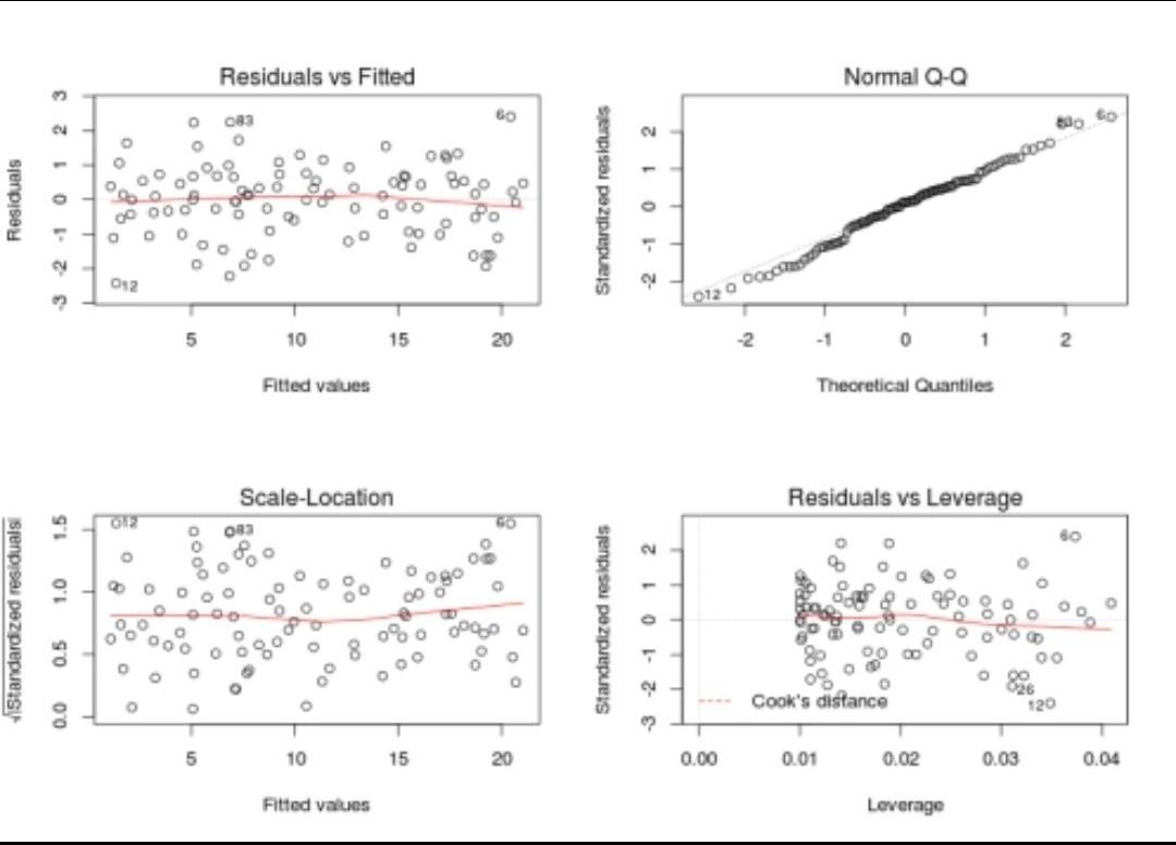
- Independent residuals and the constant residuals at every \(x\): We can check for 1 and 2 by plotting the residuals(error terms) against the fitted values (upper left graph). Generally, we should look for a lack of patterns and a consistent variance across the horizontal line.
- Normally distributed residuals: We can check for this using a couple of methods: -Q-Q-plot(upper right graph): If data is normally distributed, points should roughly align with the 45-degree line. -Boxplot: it also helps visualize outliers -Shapiro–Wilk test: If the p-value is lower than the chosen threshold, then the null hypothesis (Data is normally distributed) is rejected.
- Low multicollinearity
- You can calculate the VIF (Variable Inflation Factors) using your favorite statistical tool. If the value for each covariate is lower than 10 (some say 5), you’re good to go.
- The figure below summarizes these assumptions.
Explain briefly the K-Means clustering and how can we find the best value of K?
- K-Means is a well-known clustering algorithm. K-Means clustering is often used because it is easy to interpret and implement. It starts by partitioning a set of data into \(K\) distinct clusters and then arbitrary selects centroids of each of these clusters. It iteratively updates partitions by first assigning the points to the closet cluster and then updating the centroid and then repeating this process until convergence. The process essentially minimizes the total inter-cluster variation across all clusters.
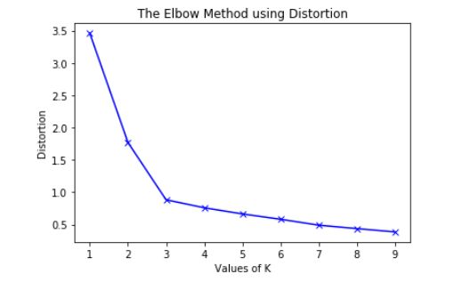
- The elbow method is a well-known method to find the best value of \(K\) in K-means clustering. The intuition behind this technique is that the first few clusters will explain a lot of the variation in the data, but past a certain point, the amount of information added is diminishing. Looking at the graph below of the explained variation (on the y-axis) versus the number of cluster \(K\) (on the x-axis), there should be a sharp change in the y-axis at some level of \(K\). For example in the graph below the drop-off is at \(k=3\).
- The explained variation is quantified by the within-cluster sum of squared errors. To calculate this error notice, we look for each cluster at the total sum of squared errors using Euclidean distance.
- Another popular alternative method to find the value of \(K\) is to apply the silhouette method, which aims to measure how similar points are in its cluster compared to other clusters. It can be calculated with this equation: \((x-y)/max(x,y)\), where \(x\) is the mean distance to the examples of the nearest cluster, and \(y\) is the mean distance to other examples in the same cluster. The coefficient varies between -1 and 1 for any given point. A value of 1 implies that the point is in the right cluster and the value of -1 implies that it is in the wrong cluster. By plotting the silhouette coefficient on the y-axis versus each \(K\) we can get an idea of the optimal number of clusters. However, it is worthy to note that this method is more computationally expensive than the previous one.
Explain what is information gain and entropy in the context of decision trees?
- Entropy and Information Gain are two key metrics used in determining the relevance of decision making when constructing a decision tree model and to determine the nodes and the best way to split.
- The idea of a decision tree is to divide the data set into smaller data sets based on the descriptive features until we reach a small enough set that contains data points that fall under one label.
- Entropy is the measure of impurity, disorder, or uncertainty in a bunch of examples. Entropy controls how a Decision Tree decides to split the data. Information gain calculates the reduction in entropy or surprise from transforming a dataset in some way. It is commonly used in the construction of decision trees from a training dataset, by evaluating the information gain for each variable, and selecting the variable that maximizes the information gain, which in turn minimizes the entropy and best splits the dataset into groups for effective classification.
Mention three ways to handle missing or corrupted data in adataset?
-
In general, real-world data often has a lot of missing values. The cause of missing values can be data corruption or failure to record data. The handling of missing data is very important during the preprocessing of the dataset as many machine learning algorithms do not support missing values. However, you should start by asking the data owner/stakeholder about the missing or corrupted data. It might be at the data entry level, because of file encoding, etc. which if aligned, can be handled without the need to use advanced techniques.
-
There are different ways to handle missing data, we will discuss only three of them:
-
Deleting the row with missing values
- The first method to handle missing values is to delete the rows or columns that have null values. This is an easy and fast method and leads to a robust model, however, it will lead to the loss of a lot of information depending on the amount of missing data and can only be applied if the missing data represent a small percentage of the whole dataset.
-
Using learning algorithms that support missing values
- Some machine learning algorithms are robust to missing values in the dataset. The K-NN algorithm can ignore a column from a distance measure when there are missing values. Naive Bayes can also support missing values when making a prediction. Another algorithm that can handle a dataset with missing values or null values is the random forest model and Xgboost (check the post in the first comment), as it can work on non-linear and categorical data. The problem with this method is that these models’ implementation in the scikit-learn library does not support handling missing values, so you will have to implement it yourself.
-
Missing value imputation
- Data imputation means the substitution of estimated values for missing or inconsistent data in your dataset. There are different ways to estimate the values that will replace the missing value. The simplest one is to replace the missing value with the most repeated value in the row or the column. Another simple way is to replace it with the mean, median, or mode of the rest of the row or the column. This advantage of this is that it is an easy and fast way to handle the missing data, but it might lead to data leakage and does not factor the covariance between features. A better way is to use a machine learning model to learn the pattern between the data and predict the missing values, this is a very good method to estimate the missing values that will not lead to data leakage and will factor the covariance between the feature, the drawback of this method is the computational complexity especially if your dataset is large.
-
Strategies for Mitigating the Impact of Outliers in Model Training
- Implementing Regularization Techniques:
- L1 (Lasso) and L2 (Ridge) regularization methods are effective for reducing overfitting, which can be exacerbated by outliers. They work by adding a penalty to the loss function that discourages large weights in the model, thus attenuating the influence of outliers. L1 regularization can also promote sparsity, which may altogether eliminate the impact of some outlier-influenced features.
- Utilizing Tree-Based Algorithms:
- Models like Random Forests and Gradient Boosting Decision Trees inherently possess a higher tolerance to outliers. They don’t rely on the assumption of data being normally distributed since they use hierarchical splitting. Outliers tend to end up in nodes that don’t significantly skew the majority of the data, thereby isolating their influence.
- Applying Log Transformations:
- For datasets where the target variable shows an exponential growth pattern, log transformation can normalize the scale, bringing the data closer to a normal distribution. This can be particularly useful when dealing with right-skewed data, as it dampens the effect of very large values. However, this technique should only be applied when it makes sense for the data distribution and the nature of the variables involved.
- Employing Robust Evaluation Metrics:
- Instead of relying on metrics that are highly sensitive to outliers, such as the Mean Squared Error, switching to more robust alternatives like the Mean Absolute Error or Median Absolute Deviation can provide a more reliable measure of model performance in outlier-affected datasets.
- Outlier Detection and Removal:
- In cases where outliers do not contribute to predictive power, especially when they result from errors or noise, it may be justifiable to remove them. This should be done with caution, considering the risk of losing valuable information. Outlier removal should always be backed by a solid rationale that aligns with the overall modeling goals and data understanding. - By combining these strategies, you can significantly reduce the adverse effects that outliers might have on your predictive models, leading to more robust and reliable outcomes.
What is an activation function and discuss the use of an activation function? Explain three different types of activation functions?
- In mathematical terms, the activation function serves as a gate between the current neuron input and its output, going to the next level. Basically, it decides whether neurons should be activated or not. It is used to introduce non-linearity into a model.
- Activation functions are added to introduce non-linearity to the network, it doesn’t matter how many layers or how many neurons your net has, the output will be linear combinations of the input in the absence of activation functions. In other words, activation functions are what make a linear regression model different from a neural network. We need non-linearity, to capture more complex features and model more complex variations that simple linear models can not capture.
- There are a lot of activation functions:
- Sigmoid function: \(f(x) = 1/(1+exp(-x))\).
- The output value of it is between 0 and 1, we can use it for classification. It has some problems like the gradient vanishing on the extremes, also it is computationally expensive since it uses exp.
- ReLU: \(f(x) = max(0,x)\).
- it returns 0 if the input is negative and the value of the input if the input is positive. It solves the problem of vanishing gradient for the positive side, however, the problem is still on the negative side. It is fast because we use a linear function in it.
- Leaky ReLU:
- Sigmoid function: \(f(x) = 1/(1+exp(-x))\).
- It solves the problem of vanishing gradient on both sides by returning a value “a” on the negative side and it does the same thing as ReLU for the positive side.
- Softmax: it is usually used at the last layer for a classification problem because it returns a set of probabilities, where the sum of them is 1. Moreover, it is compatible with cross-entropy loss, which is usually the loss function for classification problems.
Dimensionality reduction techniques
-
Dimensionality reduction techniques help deal with the curse of dimensionality. Some of these are supervised learning approaches whereas others are unsupervised. Here is a quick summary:
- PCA - Principal Component Analysis is an unsupervised learning approach and can Handle skewed data easily for dimensionality reduction.
- LDA - Linear Discriminant Analysis is also a dimensionality reduction technique based on eigenvectors but it also maximizes class separation while doing so. Moreover, it is a supervised Learning approach and it performs better with uniformly distributed data.
- ICA - Independent Component Analysis aims to maximize the statistical independence between variables and is a Supervised learning approach.
- MDS - Multi dimensional scaling aims to preserve the Euclidean pairwise distances. It is an Unsupervised learning approach.
- ISOMAP - Also known as Isometric Mapping is another dimensionality reduction technique which preserves geodesic pairwise distances. It is an unsupervised learning approach. It can handle noisy data well.
- t-SNE - Called the t-distributed stochastic neighbor embedding preserves local structure and is an Unsupervised learning approach.
What do you do when you have a low amount of data and large amount of features
- When handling a low amount of data with a large number of features:
-
Use data augmentation to create more training samples, employing techniques like geometric transformations or noise injection, but avoid excessive augmentation that can lead to misleading patterns.
-
Apply dimensionality reduction to address the curse of dimensionality, using feature selection to discard less important features and feature extraction methods like PCA to transform the feature space.
-
Reduce overfitting by minimizing the number of features, which can also improve the model’s ability to generalize and increase computational efficiency.
-
Ensure data quality, as noisy or inconsistent data can significantly impact model performance, especially when the data is scarce.
-
Implement models adept at handling high-dimensional data, like deep neural networks or ensemble methods, but be cautious of overfitting and higher computational demands.
-
Decorrelate features using Pearson correlation for linear relationships and Spearman correlation for monotonic relationships, setting a threshold to identify and eliminate redundant features.
-
Combine correlation-based feature selection with other methods for a thorough feature engineering process, and choose the correlation measure that best fits the nature of your data and analysis goals.
Sample size
- Sample size refers to the number of data points or observations in the entire dataset. It represents the total amount of data available for training, validation, and testing. The sample size is a characteristic of the dataset itself and remains fixed throughout the training process.
- Population size: Consider the size of the population you are trying to make inferences about. If the population is small, you may need a larger sample size to obtain reliable estimates. Conversely, if the population is large, a smaller sample size might be sufficient.
- Desired level of precision: Determine the level of precision or margin of error that you are willing to tolerate in your estimates. A smaller margin of error requires a larger sample size.
- Confidence level: Specify the desired level of confidence in your estimates. Commonly used confidence levels are 95% or 99%. Higher confidence levels generally require larger sample sizes.
- Variability of the data: Consider the variability or dispersion of the data you are working with. If the data points are highly variable, you may need a larger sample size to capture the underlying patterns accurately.
- Statistical power: If you are conducting hypothesis tests or performing statistical analyses, you need to consider the statistical power of your study. Higher statistical power often necessitates a larger sample size to detect meaningful effects or differences.
- Available resources: Take into account the resources available to collect and analyze data. If there are limitations in terms of time, cost, or manpower, you may need to make trade-offs and choose a sample size that is feasible within those constraints.
- Prior research or pilot studies: If prior research or pilot studies have been conducted on a similar topic, they can provide insights into the expected effect sizes and variability, which can guide sample size determination.
- Nonlinear algorithms (ANN, SVN, Random Forest), which have the ability to learn complex relationships between input and output features, often require a larger amount of training data compared to linear algorithms. These nonlinear algorithms, such as random forests or artificial neural networks, are more flexible and have higher variance, meaning their predictions can vary based on the specific data used for training.
- For example, if a linear algorithm achieves good performance with a few hundred examples per class, a nonlinear algorithm may require several thousand examples per class to achieve similar performance. Deep learning methods, a type of nonlinear algorithm, can benefit from even larger amounts of data, as they have the potential to further improve their performance with more training examples
- Also note, more data never hurts!
Define correlation
- Correlation is the degree to which two variables are linearly related. This is an important step in bi-variate data analysis. In the broadest sense correlation is actually any statistical relationship, whether causal or not, between two random variables in bivariate data.
An important rule to remember is that Correlation doesn’t imply causation.
- Let’s understand through two examples as to what it actually implies.
- The consumption of ice-cream increases during the summer months. There is a strong correlation between the sales of ice-cream units. In this particular example, we see there is a causal relationship also as the extreme summers do push the sale of ice-creams up.
- Ice-creams sales also have a strong correlation with shark attacks. Now as we can see very clearly here, the shark attacks are most definitely not caused due to ice-creams. So, there is no causation here.
- Hence, we can understand that the correlation doesn’t ALWAYS imply causation!
What is a Correlation Coefficient?
- A correlation coefficient is a statistical measure of the strength of the relationship between the relative movements of two variables. The values range between -1.0 and 1.0. A correlation of -1.0 shows a perfect negative correlation, while a correlation of 1.0 shows a perfect positive correlation. A correlation of 0.0 shows no linear relationship between the movement of the two variables.
Explain Pearson’s Correlation Coefficient
-
Wikipedia Definition: In statistics, the Pearson correlation coefficient also referred to as Pearson’s r or the bivariate correlation is a statistic that measures the linear correlation between two variables X and Y. It has a value between +1 and −1. A value of +1 is a total positive linear correlation, 0 is no linear correlation, and −1 is a total negative linear correlation.
-
Important Inference to keep in mind: The Pearson correlation can evaluate ONLY a linear relationship between two continuous variables (A relationship is linear only when a change in one variable is associated with a proportional change in the other variable)
-
Example use case: We can use the Pearson correlation to evaluate whether an increase in age leads to an increase in blood pressure.
-
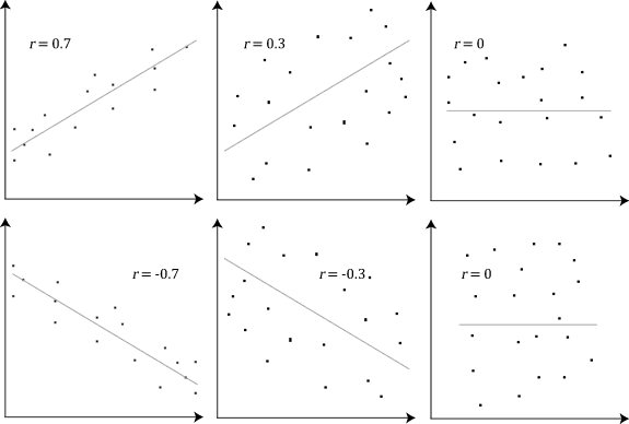
Below is an example (source: Wikipedia) of how the Pearson correlation coefficient (r) varies with the strength and the direction of the relationship between the two variables. Note that when no linear relationship could be established (refer to graphs in the third column), the Pearson coefficient yields a value of zero.
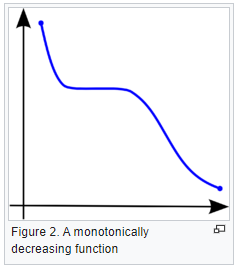
Explain Spearman’s Correlation Coefficient
-
Wikipedia Definition: In statistics, Spearman’s rank correlation coefficient or Spearman’s ρ, named after Charles Spearman is a nonparametric measure of rank correlation (statistical dependence between the rankings of two variables). It assesses how well the relationship between two variables can be described using a monotonic function.
-
Important Inference to keep in mind: The Spearman correlation can evaluate a monotonic relationship between two variables — Continous or Ordinal and it is based on the ranked values for each variable rather than the raw data.
-
What is a monotonic relationship?
- A monotonic relationship is a relationship that does one of the following:
- As the value of one variable increases, so does the value of the other variable, OR,
- As the value of one variable increases, the other variable value decreases.
- But, not exactly at a constant rate whereas in a linear relationship the rate of increase/decrease is constant.
- A monotonic relationship is a relationship that does one of the following:
- Example use case: Whether the order in which employees complete a test exercise is related to the number of months they have been employed or correlation between the IQ of a person with the number of hours spent in front of TV per week.
Compare Pearson and Spearman coefficients
- The fundamental difference between the two correlation coefficients is that the Pearson coefficient works with a linear relationship between the two variables whereas the Spearman Coefficient works with monotonic relationships as well.
- One more difference is that Pearson works with raw data values of the variables whereas Spearman works with rank-ordered variables.
- Now, if we feel that a scatterplot is visually indicating a “might be monotonic, might be linear” relationship, our best bet would be to apply Spearman and not Pearson. No harm would be done by switching to Spearman even if the data turned out to be perfectly linear. But, if it’s not exactly linear and we use Pearson’s coefficient then we’ll miss out on the information that Spearman could capture.
-
Let’s look at some examples (source: A comparison of the Pearson and Spearman correlation methods):
- Pearson = +1, Spearman = +1:
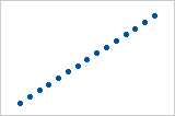
- Pearson = +0.851, Spearman = +1 (This is a monotonically increasing relationship, thus Spearman is exactly 1)
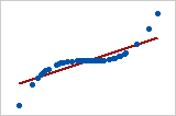
- Pearson = −0.093, Spearman = −0.093
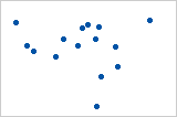
- Pearson = −1, Spearman = −1
- Pearson = −0.799, Spearman = −1 (This is a monotonically decreasing relationship, thus Spearman is exactly 1)
- Note that both of these coefficients cannot capture any other kind of non-linear relationships. Thus, if a scatterplot indicates a relationship that cannot be expressed by a linear or monotonic function, then both of these coefficients must not be used to determine the strength of the relationship between the variables.
How to choose between Pearson and Spearman correlation?
-
If you want to explore your data it is best to compute both, since the relation between the Spearman (S) and Pearson (P) correlations will give some information. Briefly, \(S\) is computed on ranks and so depicts monotonic relationships while \(P\) is on true values and depicts linear relationships.
-
As an example, if you set:
x=(1:100);
y=exp(x);                         % then,
corr(x,y,'type','Spearman');      % will equal 1, and
corr(x,y,'type','Pearson');       % will be about equal to 0.25
- This is because \(y\) increases monotonically with \(x\) so the Spearman correlation is perfect, but not linearly, so the Pearson correlation is imperfect.
corr(x,log(y),'type','Pearson'); % will equal 1
- Doing both is interesting because if you have \(S > P\), that means that you have a correlation that is monotonic but not linear. Since it is good to have linearity in statistics (it is easier) you can try to apply a transformation on \(y\) (such a log).
Multicollinearity
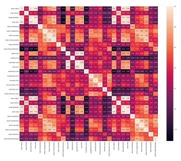
- Multicollinearity refers to the high correlation between input features in a dataset, which can adversely affect the performance of machine learning models. To identify multicollinearity, one can calculate the Pearson correlation coefficient or the Spearman correlation coefficient between the input features. The Pearson correlation coefficient measures the linear relationship between variables, while the Spearman correlation coefficient assesses the monotonic relationship between variables.
- Creating a heatmap by visualizing the correlation coefficients of input features can effectively reveal multicollinearity. In the heatmap, lighter colors indicate a high correlation, while darker colors indicate a low correlation.
- To mitigate multicollinearity, one approach is to employ Principal Component Analysis (PCA) as a data preprocessing step. PCA leverages the existing correlations among input features to combine them into a new set of uncorrelated features. By applying PCA, multicollinearity can be automatically addressed. After PCA transformation, a new heatmap can be generated to confirm the reduced correlation among the transformed features.
- For a practical demonstration of removing multicollinearity using PCA, you may refer to the article “How do you apply PCA to Logistic Regression to remove Multicollinearity?” to gain hands-on experience in its application.
- (Source image)
Mention three ways to make your model robust to outliers?
-
Investigating the outliers is always the first step in understanding how to treat them. After you understand the nature of why the outliers occurred you can apply one of the several methods mentioned below.
-
Add regularization that will reduce variance, for example, L1 or L2 regularization.
-
Use tree-based models (random forest, gradient boosting ) that are generally less affected by outliers.
-
Winsorize the data. Winsorizing or winsorization is the transformation of statistics by limiting extreme values in the statistical data to reduce the effect of possibly spurious outliers. In numerical data, if the distribution is almost normal using the Z-score we can detect the outliers and treat them by either removing or capping them with some value. If the distribution is skewed using IQR we can detect and treat it by again either removing or capping it with some value. In categorical data check for value_count in the percentage if we have very few records from some category, either we can remove it or can cap it with some categorical value like others.
-
Transform the data, for example, you do a log transformation when the response variable follows an exponential distribution or is right-skewed.
-
Use more robust error metrics such as MAE or Huber loss instead of MSE.
-
Remove the outliers, only do this if you are certain that the outliers are true anomalies that are not worth adding to your model. This should be your last consideration since dropping them means losing information.
What are L1 and L2 regularization? What are the differences between the two?
- Regularization is a technique used to avoid overfitting by trying to make the model more simple. One way to apply regularization is by adding the weights to the loss function. This is done in order to consider minimizing unimportant weights. In L1 regularization we add the sum of the absolute of the weights to the loss function. In L2 regularization we add the sum of the squares of the weights to the loss function.
- So both L1 and L2 regularization are ways to reduce overfitting, but to understand the difference it’s better to know how they are calculated:
- Loss (L2) : Cost function + \(L\) * \(weights^2\)
- Loss (L1) : Cost function + \(L\) * \(\|weights\|\)
- Where \(L\) is the regularization parameter
- L2 regularization penalizes huge parameters preventing any of the single parameters to get too large. But weights never become zeros. It adds parameters square to the loss. Preventing the model from overfitting on any single feature.
- L1 regularization penalizes weights by adding a term to the loss function which is the absolute value of the loss. This leads to it removing small values of the parameters leading in the end to the parameter hitting zero and staying there for the rest of the epochs. Removing this specific variable completely from our calculation. So, It helps in simplifying our model. It is also helpful for feature selection as it shrinks the coefficient to zero which is not significant in the model.
What are the Bias and Variance in a Machine Learning Model and explain the bias-variance trade-off?
-
The goal of any supervised machine learning model is to estimate the mapping function (f) that predicts the target variable (y) given input (x). The prediction error can be broken down into three parts:
-
Bias: The bias is the simplifying assumption made by the model to make the target function easy to learn. Low bias suggests fewer assumptions made about the form of the target function. High bias suggests more assumptions made about the form of the target data. The smaller the bias error the better the model is. If the bias error is high, this means that the model is underfitting the training data.
-
Variance: Variance is the amount that the estimate of the target function will change if different training data was used. The target function is estimated from the training data by a machine learning algorithm, so we should expect the algorithm to have some variance. Ideally, it should not change too much from one training dataset to the next, meaning that the algorithm is good at picking out the hidden underlying mapping between the inputs and the output variables. If the variance error is high this indicates that the model overfits the training data.
-
Irreducible error: It is the error introduced from the chosen framing of the problem and may be caused by factors like unknown variables that influence the mapping of the input variables to the output variable. The irreducible error cannot be reduced regardless of what algorithm is used.
-
-
The goal of any supervised machine learning algorithm is to achieve low bias and low variance. In turn, the algorithm should achieve good prediction performance. The parameterization of machine learning algorithms is often a battle to balance out bias and variance.
- For example, if you want to predict the housing prices given a large set of potential predictors. A model with high bias but low variance, such as linear regression will be easy to implement, but it will oversimplify the problem resulting in high bias and low variance. This high bias and low variance would mean in this context that the predicted house prices are frequently off from the market value, but the value of the variance of these predicted prices is low.
- On the other side, a model with low bias and high variance such as a neural network will lead to predicted house prices closer to the market value, but with predictions varying widely based on the input features.
Feature Scaling
- Feature scaling is a preprocessing step in machine learning that aims to bring all features or variables to a similar scale or range. It is essential because many machine learning algorithms perform better when the features are on a similar scale. Here are some common techniques for feature scaling:
1) Standardization (Z-score normalization): This technique scales the features to have zero mean and unit variance. It transforms the data so that it follows a standard normal distribution. Standardization is useful when the features have different scales and the algorithm assumes a Gaussian distribution.
2) Normalization (Min-Max scaling): This technique scales the features to a specific range, usually between 0 and 1. It preserves the relative relationships between data points. Normalization is suitable when the data does not follow a Gaussian distribution and the algorithm does not make assumptions about the distribution.
3) Logarithmic Transformation: This technique applies a logarithmic function to the data. It is useful when the data is skewed or has a wide range of values. Logarithmic transformation can help in reducing the impact of outliers and making the data more normally distributed.
4) Robust Scaling: This technique scales the features based on their interquartile range (IQR). It is similar to standardization but uses the median and IQR instead of the mean and standard deviation. Robust scaling is more resistant to outliers compared to standardization.
When working with AWS, you can use the following toolings for feature scaling:
-
Amazon SageMaker Data Wrangler: It provides built-in transformations for feature scaling, including standardization and normalization. You can preprocess your data using Data Wrangler’s visual interface or through its Python SDK.
-
AWS Glue: It is a fully managed extract, transform, and load (ETL) service. Glue allows you to create and execute data transformation jobs using Apache Spark. You can leverage Spark’s capabilities to perform feature scaling along with other preprocessing steps.
-
Amazon Athena: Athena is an interactive query service that allows you to query data directly from your data lake. You can use SQL queries to perform feature scaling operations within your queries, applying functions like standardization or normalization.
-
These tools provide efficient ways to preprocess and scale your features, enabling you to prepare your data for machine learning tasks effectively.
Metrics
Precision
- Definition: Precision is the ratio of true positive predictions to the total predicted positives.
- Formula: Precision = TP / (TP + FP)
- Interpretation: Measures how many of the predicted positive instances are actually positive. High precision indicates a low false positive rate.
Recall (Sensitivity)
- Definition: Recall is the ratio of true positive predictions to the total actual positives.
- Formula: Recall = TP / (TP + FN)
- Interpretation: Measures how many of the actual positive instances are correctly identified. High recall indicates a low false negative rate.
AUC-ROC (Area Under the Receiver Operating Characteristic Curve)
- Definition: AUC-ROC is a performance measurement for classification problems at various threshold settings.
- ROC Curve: Plots the true positive rate (recall) against the false positive rate (1-specificity).
- AUC Value: Represents the likelihood that the model ranks a random positive instance higher than a random negative one. A higher AUC indicates better model performance.
- Interpretation: AUC-ROC provides a single metric to compare model performance across different thresholds, with 1 being perfect and 0.5 representing random guessing.
Data
Overfitting
- Cross-Validation: Essential for evaluating model performance and ensuring generalization.
- Regularization: Effective for many models and relatively easy to implement (e.g., L1/L2 regularization).
- Early Stopping: Useful in neural networks to prevent over-training.
- Simplify the Model: Reducing complexity is a straightforward way to mitigate overfitting.
- Pruning: Specifically for decision trees and random forests, helps remove overfitted branches.
- Dropout: Specifically for neural networks, helps prevent nodes from co-adapting too much.
- Ensemble Methods: Combines multiple models to improve generalization (e.g., bagging, boosting).
- Train with More Data: If feasible, more data helps the model learn better.
- Data Augmentation: Especially useful in image processing to artificially increase dataset size.
- Feature Selection: Reduces the number of input variables, simplifying the model and reducing overfitting risks.
Underfitting
- Increase Model Complexity: Use a more complex model or add layers/neurons to a neural network to capture more intricate patterns.
- Feature Engineering: Create new features or transform existing ones to provide more relevant information to the model.
- Decrease Regularization: Reduce the strength of regularization to allow the model to fit the training data better.
- Train Longer: Ensure the model has sufficient training time to learn from the data.
- Use Different Algorithms: Experiment with more complex algorithms that might better capture the data patterns.
- Hyperparameter Tuning: Optimize the model’s hyperparameters to improve its learning capability.
- Remove Noise from Data: Clean the dataset to ensure that irrelevant or incorrect data points do not affect the model’s performance.
- Increase Training Data Quality: Improve the quality of the data rather than quantity, ensuring the data is more representative of the problem.
- Combine Models: Use ensemble methods to combine the predictions of multiple models for a stronger overall model.
- Use Pretrained Models: Leverage transfer learning by using models pretrained on similar tasks and fine-tuning them for your specific problem.
Data Imbalance:
-
Data imbalance is a common problem in machine learning where certain classes or outcomes are underrepresented in the training data. This can lead to biased models that perform well on the majority class but poorly on the minority class, simply because the model has not seen enough examples of the minority class to learn from. Data imbalance is especially problematic in applications like fraud detection or disease diagnosis, where the minority class (fraudulent transactions or positive disease cases) is often the most important to detect.
-
Strategies to address data imbalance include:
-
Resampling Techniques: Adjusting the dataset to balance the class distribution. This can be done through oversampling the minority class, undersampling the majority class, or synthesizing new data with techniques such as SMOTE (Synthetic Minority Over-sampling Technique).
-
Cost-Sensitive Learning: Modifying algorithms to make them more sensitive to the minority class by assigning higher misclassification costs to the minority class.
-
Anomaly Detection: In cases where the minority class is very rare, anomaly detection techniques might be more appropriate than standard classification methods.
-
Ensemble Methods: Using ensemble techniques such as bagging or boosting to improve the robustness of the model against the imbalance.
Long Tail Data:
-
Long tail data refers to the phenomenon where a significant portion of occurrences or events in a dataset are represented by many low-frequency, infrequent instances. In many real-world datasets, a small number of categories (the “head”) have a high number of instances, and a large number of categories (the “tail”) have a low number of instances.
-
The challenges with long tail data include:
-
Model Overfitting: The model may overfit to the head of the distribution and perform poorly on the tail instances.
-
Underrepresentation: The instances in the long tail are underrepresented, making it difficult for the model to learn from them.
- Addressing long tail issues may involve:
-
Tailored Sampling Strategies: Deliberately sampling more instances from the tail to give the model more examples to learn from.
-
Specialized Models: Developing models or components of models specifically designed to handle the long tail, such as few-shot learning techniques.
-
Transfer Learning: Using transfer learning to leverage information from related domains where data might not be as sparse.
-
Meta-Learning: Applying meta-learning approaches which train models on a variety of tasks so they can better adapt to new tasks with limited data.
- In all cases, the key to managing data imbalance, ensuring diversity, and handling long tail data is to be aware of these issues during the dataset construction, model design, and evaluation stages, and to employ strategies that mitigate their potential negative impacts on model performance.
Focal loss for imbalance class
- Focal loss is an alternative loss function to the standard cross-entropy loss used in classification problems, particularly designed to address class imbalance in datasets where there is a large discrepancy between the number of instances in each class. It was introduced by Lin et al. in the paper “Focal Loss for Dense Object Detection,” primarily for improving object detection models where the background class significantly outnumbers the object classes.
- The idea behind focal loss is to modify the cross-entropy loss so that it reduces the relative loss for well-classified examples and focuses more on hard, misclassified examples. This is achieved by adding a modulating factor to the cross-entropy loss, which down-weights the loss assigned to well-classified examples.
- The focal loss function is defined as follows:
-
Where:
- \(p_t\) is the model’s estimated probability for the class with label \(y = 1\).
- For the class labeled as \(y = 0\), the probability \(p_t\) is replaced with \((1 - p_t)\) to reflect the probability of the negative class.
- \(\alpha_t\) is a weighting factor for the class \(t\), which can be set to inverse class frequency or another vector of values to counteract class imbalance.
-
\(\gamma\) is the focusing parameter that smoothly adjusts the rate at which easy examples are down-weighted. When \(\gamma = 0\), focal loss is equivalent to cross-entropy loss. As \(\gamma\) increases, the effect of the modulating factor also increases.
- How Focal Loss Helps:
-
Balancing the Gradient: In imbalanced datasets, the majority class can dominate the gradient and cause the model to become biased towards it. Focal loss prevents this by reducing the contribution of easy examples, which typically come from the majority class, thereby allowing the model to focus on difficult examples.
-
Improving Model Performance: By concentrating on the harder examples, the model is encouraged to learn more complex features that are necessary to classify these examples correctly, often resulting in improved performance on the minority class.
-
Flexibility: The hyperparameters \(\alpha_t\) and \(\gamma\) offer flexibility to adjust the focal loss for specific problems and datasets. It allows one to balance the importance of positive/negative samples and the focusing parameter.
-
Versatility: While initially proposed for object detection tasks, focal loss has been found beneficial in various other contexts where class imbalance is a significant issue.
- In practice, focal loss has been shown to be particularly effective for training on datasets with extreme class imbalance and has been a critical component in the success of many state-of-the-art object detection models, such as RetinaNet.
Data leaks
- Data leakage occurs when preprocessing and transforming data, leading to biased and unreliable results. Two common scenarios where data leakage can occur are during feature standardization and when applying transformations to the data.
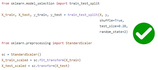
- In the case of feature standardization, data leakage happens when the entire dataset is standardized before splitting into training and test sets. This is problematic because the test set, which is derived from the full dataset, is used to calculate the mean and standard deviation for standardization. To prevent data leakage, it is recommended to perform feature standardization separately on the training and test sets after the data split.
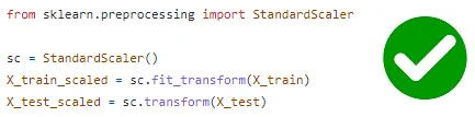
- Similarly, data leakage can occur when applying transformations to the data, such as using functions like StandardScaler or PCA. If the fit() method of these functions is called twice, once on the training set and again on the test set, new values are computed based on the test set, leading to biased results. To avoid data leakage, it is essential to call the fit() method only on the training set.
- By addressing these issues and avoiding data leakage, we can ensure the integrity and reliability of machine learning models.
- Data leakage can compromise the accuracy and generalizability of machine learning models. It is crucial to be cautious during preprocessing and transformation steps to prevent unintentional data leakage. By adhering to best practices and following proper procedures, we can minimize the risk of data leakage and obtain more robust and trustworthy results.
Data Diversity:
- Data diversity refers to the variety and representativeness of the data used to train machine learning models. Lack of diversity can lead to models that do not perform well across different groups or situations. This is a critical issue in areas like facial recognition, where a model trained on non-diverse data might fail to correctly identify faces from underrepresented groups.
- To ensure data diversity, practitioners can:
-
Collect More Representative Data: Expand data collection efforts to include a wider range of scenarios, conditions, and demographics.
-
Augmentation: Artificially expand the dataset with augmented data that has been modified in ways that are plausible in the real world, such as different lighting conditions for images or different accents in speech recognition.
-
Domain Adaptation: Adapt models trained on one domain to work on another domain, helping to generalize better across different conditions.
-
Fairness and Bias Evaluation: Use fairness metrics and bias evaluation techniques to actively measure and address issues of fairness in model predictions.
Balancing data:
- Balancing data refers to adjusting the class distribution in a dataset to ensure that each class or category is represented fairly. This is often done when there is a significant class imbalance, meaning some classes have significantly fewer samples compared to others. Balancing the data can help prevent bias and improve the performance of machine learning models.
- Here are some common techniques for balancing data:
- Oversampling: Increase the number of samples in the minority class by randomly replicating existing samples or generating synthetic samples using techniques like SMOTE (Synthetic Minority Over-sampling Technique). This helps to create a more balanced representation of classes.
- Undersampling: Decrease the number of samples in the majority class by randomly removing instances. This method aims to reduce the dominance of the majority class and increase the influence of the minority class.
- Stratified Sampling: During the dataset splitting process (e.g., train-test split or cross-validation), ensure that the ratio of different classes remains consistent in each subset. This helps maintain the class distribution across the training and evaluation phases.
- Ensemble Methods: Utilize ensemble learning techniques that combine multiple models trained on balanced subsets of the data. Each model focuses on a different subset or variation of the data to capture diverse representations.
- Cost-sensitive Learning: Assign different costs or weights to different classes during model training. This gives higher importance to underrepresented classes, forcing the model to pay more attention to them.
- Data Augmentation: Generate additional samples by applying transformations or perturbations to existing data. This technique can help increase the number of samples in the minority class, providing more training data without collecting new data.
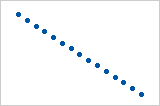
Randomness
- Randomness plays a role in machine learning models, and the random state is a hyperparameter used to control the randomness within these models. By using an integer value for the random state, we can ensure consistent results across different executions. However, relying solely on a single random state can be risky because it can significantly affect the model’s performance.
- For instance, consider the train_test_split() function, which splits a dataset into training and testing sets. The random_state hyperparameter in this function determines the shuffling process prior to the split. Depending on the random state value, different train and test sets will be generated, and the model’s performance is highly influenced by these sets.
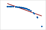
- To illustrate this, let’s look at the root mean squared error (RMSE) scores obtained from three linear regression models, where only the random state value in the train_test_split() function was changed:
- Random state = 0 → RMSE: 909.81
- Random state = 35 → RMSE: 794.15
- Random state = 42 → RMSE: 824.33
- As observed, the RMSE values vary significantly depending on the random state.
- To mitigate this issue, it is recommended to run the model multiple times with different random state values and calculate the average RMSE score. However, performing this manually can be tedious. Instead, cross-validation techniques can be employed to automate this process and obtain a more reliable estimate of the model’s performance.
- Relying on a single random state in machine learning models can yield inconsistent results, and it is advisable to leverage cross-validation methods to mitigate this issue.
Sigmoid vs Softmax
- Output Range: The sigmoid function outputs a value between 0 and 1 for each input, making it suitable for binary classification. Softmax outputs a probability distribution over multiple classes, with each value between 0 and 1 summing up to 1.
- Use Case: Sigmoid is used for binary classification tasks, where each input needs to be classified into one of two classes. Softmax is used for multi-class classification tasks, where each input is assigned to one of several classes.
- Mathematical Formulation: Sigmoid is defined as ( \sigma(x) = \frac{1}{1 + e^{-x}} ), applying independently to each input. Softmax is defined as ( \text{softmax}(x_i) = \frac{e^{x_i}}{\sum_{j} e^{x_j}} ), normalizing inputs into a probability distribution.
- Gradient Properties: Sigmoid can suffer from vanishing gradients, particularly for extreme values, which can slow down learning. Softmax, while also susceptible to gradient issues, is generally more stable for multi-class classification and allows gradients to propagate effectively across all classes.
Deep Learning
- Deep Learning (DL) is a specialized branch of machine learning that employs deep neural networks to process and make sense of vast amounts of data automatically. By learning to recognize patterns directly from data, deep learning excels in managing unstructured data such as images and text. This capability has significantly advanced fields like computer vision and natural language processing, pushing the boundaries of applications such as real-time translation and autonomous driving.
Fully Connected Network
- A fully connected layer is a neural network layer where each neuron connects to all neurons in the previous layer. It performs a linear transformation using a weight matrix and bias, followed by an activation function to introduce non-linearity.
- A fully connected network (FCN) consists entirely of FC layers and is commonly used in MLPs (Multilayer Perceptrons).
- Activation functions act as filters, determining which neurons activate, but all connections remain intact, maintaining full connectivity.
Analogy: A Fully Connected Network as a Highway System 🚗🛣️
Imagine a highway system where:
- Neurons = Intersections
- Connections (Weights) = Roads between intersections
-
Activation Function = Traffic lights controlling traffic flow
-
Each intersection (neuron) connects to all intersections in the next city (layer) via roads (weights), ensuring full connectivity. However, activation functions act as traffic lights—some roads (connections) may have a red light (inactive neuron), preventing traffic (signals), while others have a green light (active neuron), allowing data to pass.
- Even if some roads are temporarily blocked, they still exist and can be used later if the activation changes, ensuring that the network remains fully connected at all times.
Transformer differences
- Encoder-Only Models:
- Purpose: Primarily used for tasks requiring understanding or representation of input data, such as text classification and embeddings generation (e.g., BERT).
- Function: The encoder transforms the input into a dense representation (embedding) without generating sequential outputs.
- Encoder-Decoder Models:
- Purpose: Designed for sequence-to-sequence tasks, such as machine translation and text summarization, where input needs to be converted into a different sequence.
- Function: The encoder processes the input into a context vector (embedding), and the decoder generates the output sequence from this context, ensuring meaningful transformations.
- Decoder-Only Models:
- Purpose: Used for generative tasks where the model generates sequences from initial input, such as text generation and language modeling (e.g., GPT).
- Function: The decoder autoregressively generates each token in the output sequence based on the previous tokens and initial input, without an explicit encoder phase.
Why did the transition happen from RNNs to LSTMs
- Long-term Dependencies: LSTMs effectively capture long-term dependencies in sequences, addressing RNNs’ limitations in handling long-term information due to vanishing gradients.
- Gradient Issues: LSTMs mitigate the vanishing and exploding gradient problems that RNNs suffer from, ensuring stable training over long sequences.
- Memory Cells: LSTMs use memory cells and gates (input, forget, and output) to control the flow of information, allowing selective retention and forgetting, which enhances learning efficiency.
- Performance: LSTMs generally outperform RNNs in tasks involving complex temporal patterns, such as language modeling, speech recognition, and time-series prediction.
What is the difference between self attention and Bahdanau (traditional) attention
- Self-attention computes attention scores within a single sequence, allowing each element to focus on all other elements, enabling the model to capture dependencies regardless of their distance.
- Bahdanau attention (additive attention) is used in sequence-to-sequence models, where the decoder focuses on different parts of the input sequence to generate each output element, using a learned alignment mechanism to determine relevant input parts. Self-attention is typically used in models like Transformers, while Bahdanau attention is common in earlier sequence-to-sequence models like RNNs and LSTMs.
Bahdanau Attention
- Query (Q): Decoder hidden state at the current time step.
- Key (K) and Value (V): Encoder hidden states.
- Process: Compute attention scores by applying a neural network to (Q, K), use softmax to get weights, and produce a context vector by weighted sum of V.
Self-Attention
- Query (Q), Key (K), and Value (V): All derived from the same input sequence.
-
Process: Compute attention scores using dot-product of Q and K, scale, apply softmax to get weights, and produce output by weighted sum of V.
- These methods differ in their source of Q, K, and V and their application context within sequence models.
Two Tower
- Separate Towers for Users and Items: Two-tower architectures in recommendation systems consist of two neural network models, one for encoding user features and another for item features, allowing for separate and specialized processing of each type.
- Embedding Generation: Each tower generates embeddings for users and items independently, capturing their respective characteristics and preferences.
- Similarity Computation: The embeddings from the user and item towers are then compared using a similarity measure, like dot product or cosine similarity, to generate recommendations.
- Scalability and Flexibility: This architecture allows for efficient retrieval in large-scale systems, as embeddings can be precomputed and indexed, and supports flexible integration of diverse feature types for both users and items.
Why should we use Batch Normalization?
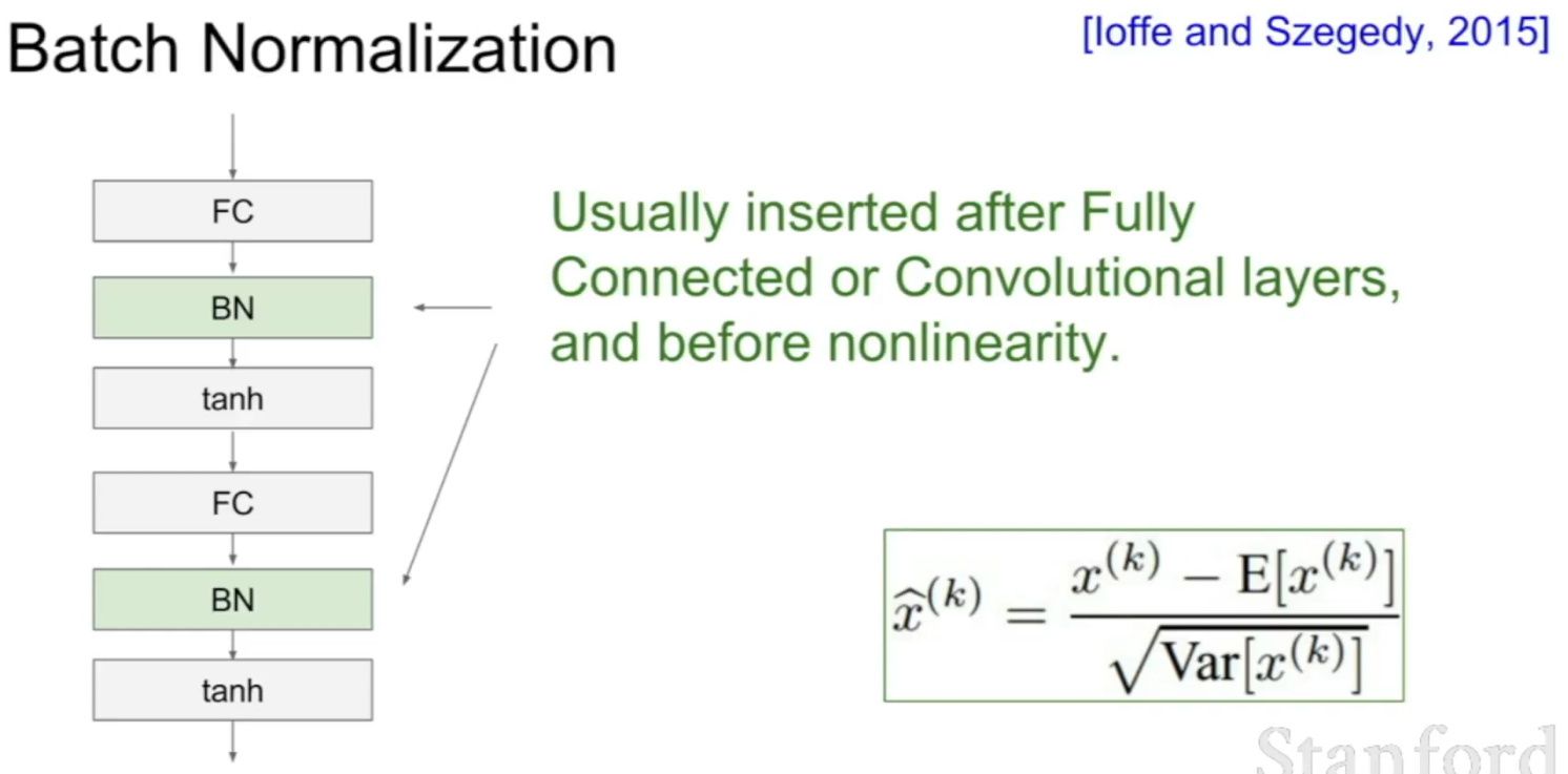
- Batch normalization is a technique for training very deep neural networks that standardizes the inputs to a layer for each mini-batch.
- Usually, a dataset is fed into the network in the form of batches where the distribution of the data differs for every batch size. By doing this, there might be chances of vanishing gradient or exploding gradient when it tries to backpropagate. In order to combat these issues, we can use BN (with irreducible error) layer mostly on the inputs to the layer before the activation function in the previous layer and after fully connected layers.
- Batch Normalisation has the following effects on the Neural Network:
- Robust Training of the deeper layers of the network.
- Better covariate-shift proof NN Architecture.
- Has a slight regularization effect.
- Centered and controlled values of Activation.
- Tries to prevent exploding/vanishing gradient.
- Faster training/convergence.
What is weak supervision?
- Weak Supervision (which most people know as the Snorkel algorithm) is an approach designed to help annotate data at scale, and it’s a pretty clever one too.
- Imagine that you have to build a content moderation system that can flag LinkedIn posts that are offensive. Before you can build a model, you’ll first have to get some data. So you’ll scrape posts. A lot of them, because content moderation is particularly data-greedy. Say, you collect 10M of them. That’s when trouble begins: you need to annotate each and every one of them - and you know that’s gonna cost you a lot of time and a lot of money!
- So you want to use autolabeling (basically, you want to apply a pre-trained model) to generate ground truth. The problem is that such a model doesn’t just lie around, as this isn’t your vanilla object detection for autonomous driving use case, and you can’t just use YOLO v5.
- Rather than seek the budget to annotate all that data, you reach out to subject matter experts you know on LinkedIn, and you ask them to give you a list of rules of what constitutes, according to each one of them, an offensive post.
Person 1's rules:
- The post is in all caps
- There is a mention of Politics

Person 2's rules:
- The post is in all caps
- It uses slang
- The topic is not professional

...

Person 20's rules:
- The post is about religion
- The post mentions death
- You then combine all rules into a mega processing engine that functions as a voting system: if a comment is flagged as offensive by at least X% of those 20 rule sets, then you label it as offensive. You apply the same logic to all 10M records and are able to annotate then in minutes, at almost no costs.
- You just used a weakly supervised algorithm to annotate your data.
- You can of course replace people’s inputs by embeddings, or some other automatically generated information, which comes handy in cases when no clear rules can be defined (for example, try coming up with rules to flag a cat in a picture).
Active learning
- Active learning is a semi-supervised ML training paradigm which, like all semi-supervised learning techniques, relies on the usage of partially labeled data.
- Active Learning consists of dynamically selecting the most relevant data by sequentially:
- selecting a sample of the raw (unannotated) dataset (the algorithm used for that selection step is called a querying strategy).
- getting the selected data annotated.
- training the model with that sample of annotated training data.
- running inference on the remaining (unannotated) data.
- That last step is used to evaluate which records should be then selected for the next iteration (called a loop). However, since there is no ground truth for the data used in the inference step, one cannot simply decide to feed the – data where the model failed to make the correct prediction, and has instead to use metadata (such as the confidence level of the prediction) to make that decision.
- The easiest and most common querying strategy used for selecting the next batch of useful data consists of picking the records with the lowest confidence level; this is called the least-confidence querying strategy, which is one of many possible querying strategies.
What is active learning?
- When you don’t have enough labeled data and it’s expensive and/or time consuming to label new data, active learning is the solution. Active learning is a semi-supervised ML training paradigm which, like all semi-supervised learning techniques, relies on the usage of partially labeled data. Active Learning helps to select unlabeled samples to label that will be most beneficial for the model, when retrained with the new sample.
- Active Learning consists of dynamically selecting the most relevant data by sequentially:
- selecting a sample of the raw (unannotated) dataset (the algorithm used for that selection step is called a querying strategy)
- getting the selected data annotated
- training the model with that sample of annotated training data
- running inference on the remaining (unannotated) data.
- That last step is used to evaluate which records should be then selected for the next iteration (called a loop). However, since there is no ground truth for the data used in the inference step, one cannot simply decide to feed the data where the model failed to make the correct prediction, and has instead to use metadata (such as the confidence level of the prediction) to make that decision.
- The easiest and most common querying strategy used for selecting the next batch of useful data consists of picking the records with the lowest confidence level; this is called the least-confidence querying strategy, which is one of many possible querying strategies. (Technically, those querying strategies are usually brute-force, arbitrary algorithms which can be replaced by actual ML models trained on metadata generated during the training and inference phases for more sophistication).
- Thus, the most important criterion is selecting samples with maximum prediction uncertainty. You can use the model’s prediction confidence to ascertain uncertain samples. Entropy is another way to measure such uncertainty. Another criterion could be diversity of the new sample with respect to exiting training data. You could also select samples close to labeled samples in the training data with poor performance. Another option could be selecting samples from regions of the feature space where better performance is desired. You could combine all the strategies in your active learning decision making process.
- The training is an iterative process. With active learning you select new sample to label, label it and retrain the model. Adding one labeled sample at a time and retraining the model could be expensive. There are techniques to select a batch of samples to label. For deep learning the most popular active learning technique is entropy with is Monte Carlo dropout for prediction probability.
- The process of deciding the samples to label could also be implemented with Multi Arm Bandit. The reward function could be defined in terms of prediction uncertainty, diversity, etc.
- Let’s go deeper and explain why the vanilla form of Active Learning, “uncertainty-based”/”least-confidence” Active Learning, actually perform poorly via real-life datasets:
- Let’s take the example of a binary classification model identifying toxic content in tweets, and let’s say we have 100,000 tweets as our dataset.
- Here is how uncertainty-based AL would work:
- We pick 1,000 (or another number, depending on how we tune the process) records - at that stage, randomly.
- We annotate that data as toxic / not-toxic.
- We train our model with it and get a (not-so-good) model.
- We use the model to infer the remaining 99,000 (unlabeled) records.
- We don’t have ground truth for those 99,000, so we can’t select which records are incorrectly predicted, but we can use metadata, such as the confidence level, as a proxy to detect bad predictions. With least confidence Active Learning, we would pick the 1,000 records predicted with the lowest confidence level as our next batch.
- Go to (2) and repeat the same steps, until we’re happy with the model.
- What we did here, is assume that confidence was a good proxy for usefulness, because it is assumed that low confidence records are the hardest for the model to learn, and hence that the model needs to see them to learn more efficiently.
- Let’s consider a scenario where it is not. Assume now that this training data is not clean, and 5% of the data is actually in Spanish. If the model (and the majority of the data) was meant to be for English, then chances are, the Spanish tweets will be inferred with a low confidence: you will actually pollute the dataset with data that doesn’t belong there. In other words, low confidence can happen for a variety of different reasons. That’s what happens when you do active learning with messy data.
- To resolve this, one solution is to stop using confidence level alone: confidence levels are just one meta-feature to evaluate usefulness.
- In a nutshell, active learning is an incremental semi-supervised learning paradigm where training data is selected incrementally and the model is sequentially retrained (loop after loop), until either the model reaches a specific performance or labeling budget is exhausted.
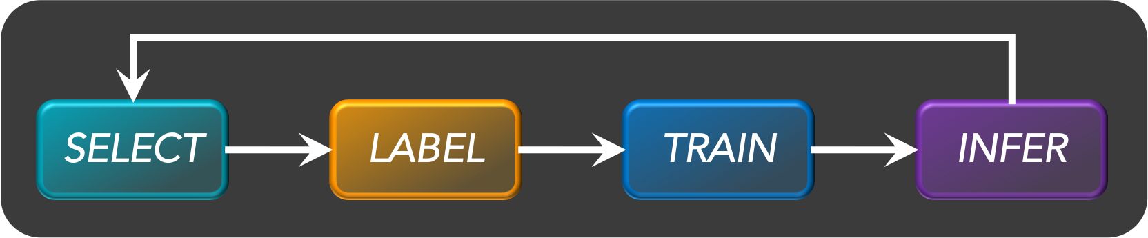
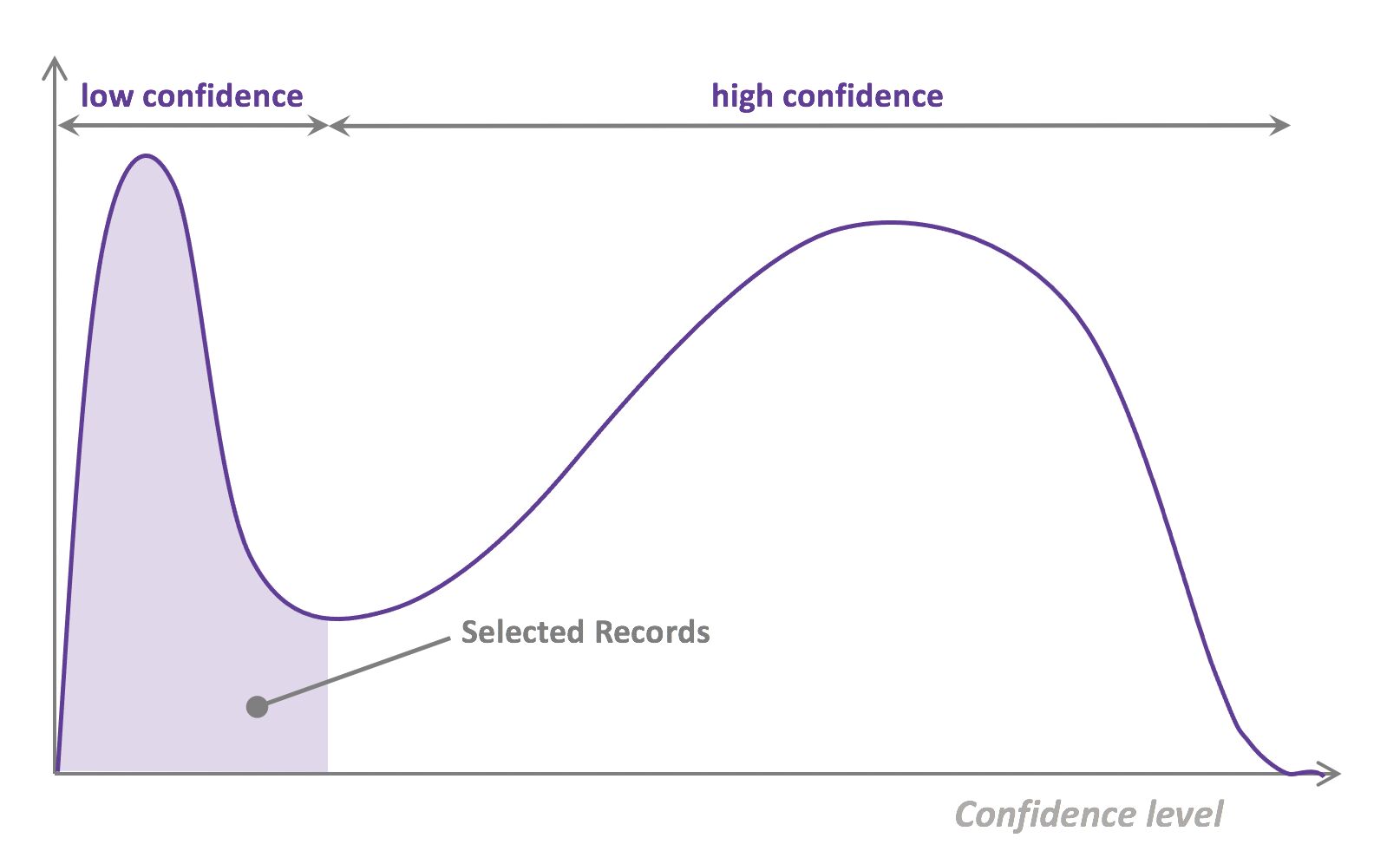
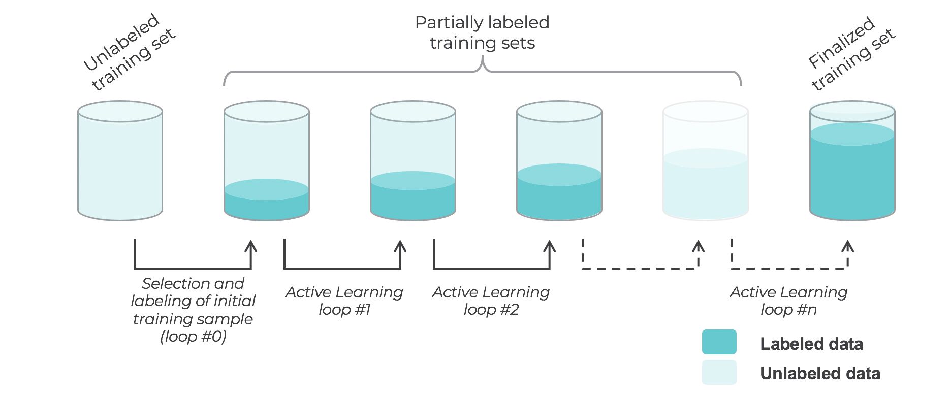
What are the types of active learning?
- There are many different “flavors” of active learning, but did you know that active learning could be broken down into two main categories, “streaming active learning”, and “pooling (batch) active learning”?
- Pooling Active Learning, is when all records available for training data have to be evaluated before a decision can be made about the ones to keep. For example, if your querying strategy is least-confidence, you goal is to select the N records that were predicted with the lowest confidence level in the previous loop, which means all records have to be ranked accordingly to their confidence level. Pooling Active Learning hence requires more compute resources for inference (the entire remainder of the dataset, at each loop, needs to be inferred), but provides a better control of loop sizes and the process as a whole.
- Streaming Active Learning, is when a decision is made “on the fly”, record by record. If your selection strategy was to select all records predicted with a confidence level lower than X% for the previous loop, you’d be doing Streaming AL. This technique obviously requires less compute, and can be used in combination with Online Learning, but it comes with a huge risk: there is no guarantee regarding the amount of data that will be selected. Set the threshold too low, and you won’t select any data for the next loop. Set the threshold too high, and all the remaining data gets selected, and you lose the benefit of AL.
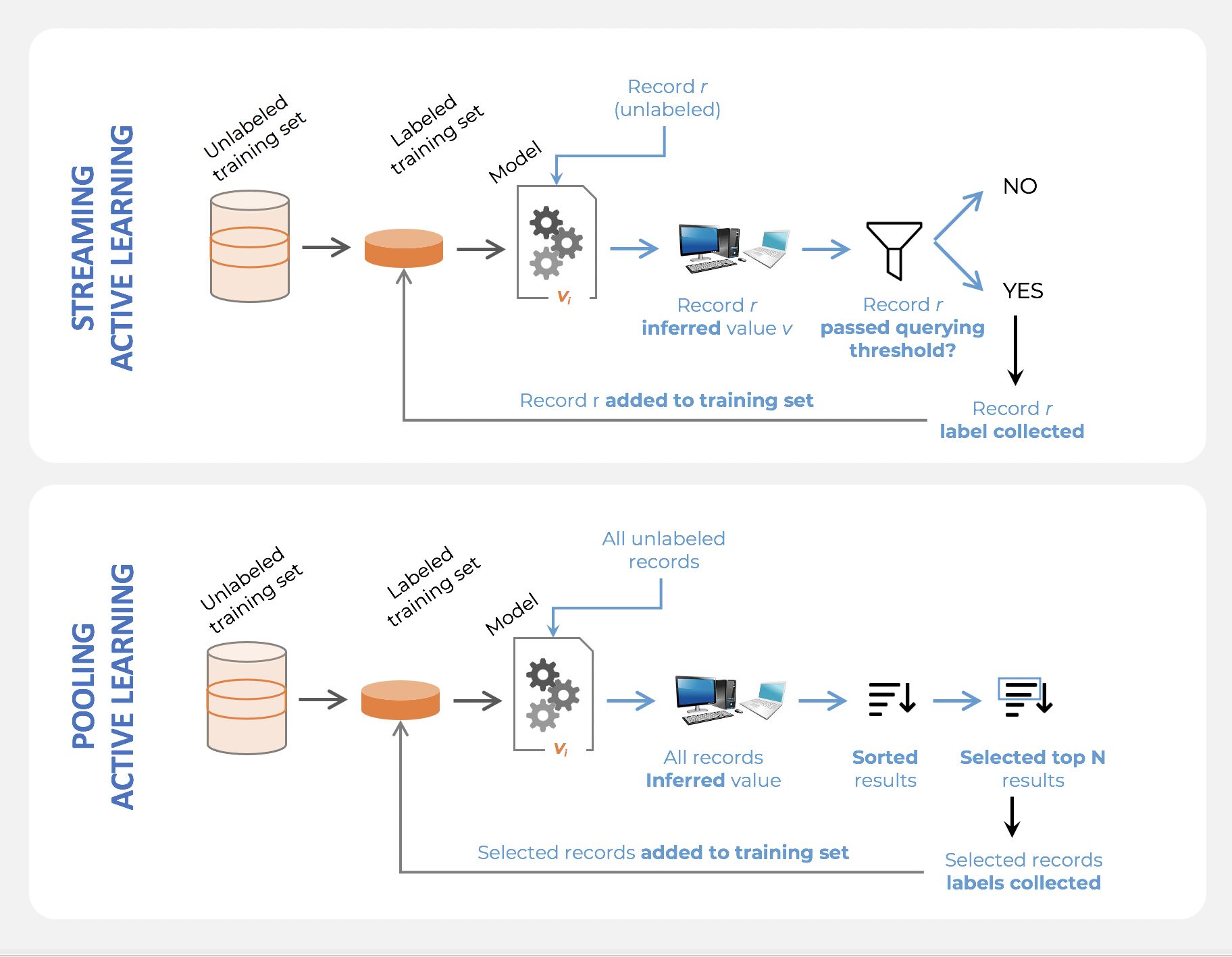
What is the difference between online learning and active learning?
- Online learning is essentially the concept of training a machine learning model on streaming data. In that case, data arrives little-by-little, sequentially, and the model is updated as opposed to be trained entirely from scratch.
- Active learning also consists in training a model sequentially, but the difference is that the training dataset is already fully available. Active learning simply selects small samples of data incrementally; the model is either retrained with the totality of selected records at a given point in time, or updated with the newly selected data.
- Online learning is required when models are to be trained at the point of collection (e.g, on the edge of a device), but active learning, just like supervised learning, usually involves the model being trained offline.
Why is active learning not frequently used with deep learning?
-
Active Learning was relatively popular among ML scientists during the pre-Deep Learning era, and somehow fell out of favor afterwards.
-
The reason why is actually relatively simple: Active Learning usually doesn’t work as well with Deep Learning Models (at least the most common querying strategies don’t). So people gave up on Deep Active Learning pretty quickly. The two most important reasons are the following:
-
The least-confidence, by far the most popular querying strategy, requires the computation of a confidence score. However, the softmax technique which most ML scientists rely on, is relatively unreliable (see this article for details to learn about a better way to compute confidence: https://arxiv.org/pdf/1706.04599.pdf)
-
Active learning, as a process, is actually meant to “grow” a better dataset dynamically. At each loop, more records are selected, which means the same model is retrained with incrementally larger data. However, many hyperparameters in neural nets are very sensitive to the amount of data used. For example, a certain number of epochs might lead to overfitting with early loops and underfitting later on. The proper way of doing Deep Active Learning would be to do hyperparameter tuning dynamically, which is rarely done.
What does active learning have to do with explore-exploit?
- Using the “uncertainty-based”/”least/lowest-confidence” querying strategy as a selection criteria in an active learning process could cause issues when working with a real-life (messy) dataset, as indicated above.
- Uncertainty-based active learning aims at selecting records based on how “certain” (or confident) the model already is about what it knows. Assuming the model can be trusted to self-evaluate properly, then:
- Selecting low confidence records is about picking what the model seems not to know yet; it is a pure exploration process.
- Selecting high confidence records is about picking what the model seems to already know, and that would be about reinforcing that knowledge; it is a pure exploitation process.
- While the “uncertainty-based”/”least/lowest-confidence” querying strategy strategy is the most common using active learning, it might be better to balance exploration and exploitation, and that active learning can and should, in fact, be formulated as a reinforcement learning problem.
What are some applications of RL beyond gaming and self-driving cars?
- Reinforcement learning is NOT just used in gaming and self-driving cars, here are three common use cases you should know in 2022:
-
Multi-arm bandit testing (MAB)
- A little bit about reinforcement learning (RL): you train an agent to interact with the environment and figure out the optimum policy which maximizes the reward (a metric you select).
- MAB is a classic reinforcement learning problem that can be used to help you find a best options out of a lot of treatments in experimentation.
- Unlike A/B tests, MAB tries to maximizes a metric (reward) during the course of the test. It usually has a lot of treatments to select from. The trade-off is that you can draw causal inference through traditional A/B testing, but it’s hard to analyze each treatment through MAB; however, because it’s dynamic, it might be faster to select the best treatment than A/B testing.
-
Recommendation engines
- While traditional matrix factorization works well for recommendation engines, using reinforcement learning can help you maximize metrics like customer engagement and metrics that measure downstream impact.
- For example, social media can use RL to maximize ‘time spent’ or ‘review score’ when recommending content; so this way, instead of just recommending similar content, you might also help customers discover new content or other popular content they like.
-
Portfolio Management
- RL has been used in finance recently as well. Data scientist can train the agent to interact with a trading environment to maximize the return of the portfolio. For example, if the agent selects an allocation of 70% stock, 10% Cash, and 20% bond, the agent gets a positive or negative reward for this allocation. Through iteration, the agent finds out the best allocation.
- Robo-advisers can also use RL to learn investors risk tolerance.
- Of course, self-driving cars, gaming, robotics use RL heavily, but I’ve seen data scientists from industries mentioned above (retail, social media, finance) start to use more RL in their day-to-day work.
You are using a deep neural network for a prediction task. After training your model, you notice that it is strongly overfitting the training set and that the performance on the test isn’t good. What can you do to reduce overfitting?
- To reduce overfitting in a deep neural network changes can be made in three places/stages: The input data to the network, the network architecture, and the training process:
- The input data to the network:
- Check if all the features are available and reliable
- Check if the training sample distribution is the same as the validation and test set distribution. Because if there is a difference in validation set distribution then it is hard for the model to predict as these complex patterns are unknown to the model.
- Check for train / valid data contamination (or leakage)
- The dataset size is enough, if not try data augmentation to increase the data size
- The dataset is balanced
- Network architecture:
- Overfitting could be due to model complexity. Question each component:
- can fully connect layers be replaced with convolutional + pooling layers?
- what is the justification for the number of layers and number of neurons chosen? Given how hard it is to tune these, can a pre-trained model be used?
- Add regularization - ridge (l1), lasso (l2), elastic net (both)
- Add dropouts
- Add batch normalization
- The training process:
- Improvements in validation losses should decide when to stop training. Use callbacks for early stopping when there are no significant changes in the validation loss and restore_best_weights.
A/B Testing
Briefly explain the A/B testing and its application? What are some common pitfalls encountered in A/B testing?
- A/B testing helps us to determine whether a change in something will cause a change in performance significantly or not. So in other words you aim to statistically estimate the impact of a given change within your digital product (for example). You measure success and counter metrics on at least 1 treatment vs 1 control group (there can be more than 1 XP group for multivariate tests).
- You should rely on experimentation to guide product development not only because it validates or invalidates your hypotheses, but, more important, because it helps create a mentality around building a minimum viable product (MVP) and exploring the terrain around it.
- With experimentation, when you make a strategic bet to bring about a drastic, abrupt change, you test to map out where you’ll land.
- So even if the abrupt change takes you to a lower point initially, you can be confident that you can hill climb from there and reach a greater height
- Used Split.io for NuAIg
- We have guardrail metrics as well to make sure the new release is not causing friction:
- Total revenue per user
- Opt out selected
- Percentage of unique users
- check every KPI and metric important to business
- Applications:
-
Consider the example of a general store that sells bread packets but not butter, for a year. If we want to check whether its sale depends on the butter or not, then suppose the store also sells butter and sales for next year are observed. Now we can determine whether selling butter can significantly increase/decrease or doesn’t affect the sale of bread.
-
While developing the landing page of a website you create 2 different versions of the page. You define a criteria for success eg. conversion rate. Then define your hypothesis,
- Null hypothesis (H): No difference between the performance of the 2 versions.
- Alternative hypothesis (H’): version A will perform better than B.
-
-
Note that you will have to split your traffic randomly (to avoid sample bias) into 2 versions. The split doesn’t have to be symmetric, you just need to set the minimum sample size for each version to avoid undersample bias.
-
Now if version A gives better results than version B, we will still have to statistically prove that results derived from our sample represent the entire population. Now one of the very common tests used to do so is 2 sample t-test where we use values of significance level (alpha) and p-value to see which hypothesis is right. If p-value<alpha, H is rejected.
- Common pitfalls:
- Wrong success metrics inadequate to the business problem
- Lack of counter metric, as you might add friction to the product regardless along with the positive impact
- Sample mismatch: heterogeneous control and treatment, unequal variances
- Underpowered test: too small sample or XP running too short 5. Not accounting for network effects (introduce bias within measurement)
Best practices for A/B Testing
- Taken from here
- Measure one change at a time.
- This is not to say that you can only test one thing at a time, but that you have to design your experiment properly so that you are able to measure one change at a time. At LinkedIn, a product launch usually involves multiple features/components. One big upgrade to LinkedIn Search in 2013 introduced unified search across different product categories. With this functionality, the search box is smart enough to figure out query intent without explicit input on categories such as “People,” or “Jobs,” or “Companies.”
- However, that was not all. Almost every single component on the search landing-page was touched, from the left rail navigation to snippets and action buttons. The first experiment was run with all changes lumped together. To our surprise, many key metrics tanked. It was a lengthy process to bring back one feature at a time in order to figure out the true culprit. In the end, we realized that several small changes, not the unified search itself, were responsible for bringing down clicks and revenue. After restoring these features, unified search was shown to be positive to user experience and deployed to everyone.
- Decide on triggered users, but report on all users.
- It is very common that an experiment only impacts a small fraction of your user base. For example, we want to automatically help people fill in their patents on their LinkedIn profiles, but not every member has a patent. So the experiment would only be affecting those ~5% of members who have filed patents. To measure how much benefit this is bringing to our members, we have to focus on this small subsegment, the “triggered” users. Otherwise, the signal from that 5% of users would be lost in the 95% noise. However, once we determined that patents are a beneficial feature, we needed to have a “realistic” estimate of the overall impact. How is LinkedIn’s bottom line going to change once this feature is rolled out universally? Having such a “site-wide” impact not only makes it possible to compare impacts across experiments, but also easy to quantify ROI.
- The experimental group should not be influenced by the experiment outcomes.
- The fundamental assumption of A/B testing is that the difference between the A and B groups is only caused by the treatment we impose. It may be obvious that we need to make sure the users in A and B are similar enough to begin with. The standard approach to check for any pre-existing differences is to run an A/A test before the actual A/B test, where both groups of users receive identical treatments. However, it is equally important to make sure the user groups stay “similar” during the experiment especially in the online world because the experimental population is usually “dynamic”. As an example, we tested a new feature where members received a small banner on their LinkedIn profile page to encourage them to explore our new homepage. Only users who had not visited the homepage recently were eligible to be in the experiment, and the eligibility was dynamically updated after a user visited the homepage. Because the banner brought more users in the treatment group to visit the homepage, more treatment users became ineligible over time. Because these “additionally” removed users tend to be more active than the rest, we artificially created a difference between users in A and B as the test continued. In general, if the experimental population is directly influenced by the experiment outcomes, we are likely to see a bias. Such bias could void the experiment results because it usually overwhelms any real signal resulting from the treatment itself.
- Avoid coupling a marketing campaign with an A/B test.
- We have recently revamped the Who Viewed My Profile page. The product team wanted to measure through an A/B test if the changes are indeed better, and if so, by how much. The marketing team wanted to create buzz around the new page with an email campaign. This is a very common scenario, but how can the A/B test and the email campaign coexist? Clearly, we can only send campaign emails to the treatment group, since there is nothing new for members in control. However, such a campaign would contaminate the online A/B test because it encourages more members from the treatment to visit. These additional users tend to be less engaged, therefore we are likely to see an artificial drop in key metrics. It is best to measure the A/B test first before launching the campaign.
- Use a simple rule of thumb to address multiple testing problems.
- Multiple testing problems are extremely prevalent in online A/B testing. The symptom is that irrelevant metrics appear to be statistically significant. The root cause is usually because too many metrics are examined simultaneously (keep in mind that we compute over 1000 metrics for each experiment). Even though we have tried to educate people on the topic of multiple testing, many are still clueless about what they should do when a metric is unexpectedly significant. Should they trust it or treat it as noise? Instead, we have found it very effective to introduce a simple rule of thumb: Use the standard 0.05 p-value cutoff for metrics that are expected to be impacted, but use a smaller cutoff, say 0.001, for metrics that are not. The rule-of-thumb is based on an interesting Bayesian interpretation. It boils down to how much we believe a metric will be impacted before we even run the experiment. In particular, if using 0.05 reflects a prior probability of 50%, then using 0.001 means a much weaker belief - at about 2%.
- These are only a few best practices for experimentation, but they’ve proven crucial for product development at LinkedIn. As I’ve said before, A/B testing and making data driven decisions through experimentation is an extremely important part of the culture at LinkedIn. It guides how and why we build products for our users by giving us crucial data on how they actually use our services. By following these five lessons, developers across all companies and industries can not only make more informed decisions about their products, but also create a better experience for the people using them.
Small file and big file problem in Big data
- The “small file problem” is kind of notorious in the big data space.
- Did you know there’s also the “Big/large file problem”?
- Say you have a billion records. The small file problem would be like.. 10 records per file and 100 million files. Combining all these files is slow, terrible, and has made many data engineers cry.
- The large file problem would be the opposite problem. 1 billion records in 1 file. This is also a huge problem because how do you parallelize 1 file? You can’t without splitting it up first.
- To avoid crying, the solution is sizing your files the right way. Aiming for between 100-200 MBs for file is usually best. In this contrived example, you’d have a 1000 files each with 1 million records.
- It is worth seeing the spread of files and the size and understanding what optimal file size works out best.
- Too low and you have the risk of more files, too high and the parallelism isn’t going to be effective.
- It is recommended to understand up parallelism, and block size and seeing how the distribution of your data (in files) is before adding an arbitrary default file size value.
Comparing Group Normalization and Batch Normalization
-
Batch Normalization (BN) and Group Normalization (GN) are techniques utilized to streamline the training of Deep Neural Networks (DNNs). They tackle the issue of internal covariate shift, which is the variation in the distribution of network layer inputs as the network parameters are updated during training.
- Understanding Internal Covariate Shift:
- Internal covariate shift describes the phenomenon where the statistical properties, such as mean and variance, of a layer’s inputs shift during training, which can slow down the learning process and complicate the convergence of the network. For instance, in a deep learning model for a recommender system, the input data features evolve across layers from simple, easily identifiable attributes to more complex, abstract patterns. If these evolving features shift too much statistically, it can destabilize the learning process, making it difficult for the model to develop stable, representative features. This shift can necessitate fine-tuning hyperparameters, potentially leading to longer training times and a challenging optimization landscape.
- Batch Normalization Process:
- BN standardizes the inputs to a layer for each mini-batch. This entails calculating the mean and variance for the batch and then using these statistics to normalize the batch’s data. Post-normalization, the data are scaled and shifted based on parameters that the network learns during training. This standardization is computed for each feature independently and relies on the statistics of the entire batch, thereby potentially causing issues when working with smaller batch sizes or when batch data is not representative of the overall dataset.
- Group Normalization Explained:
- GN divides the input channels into groups and normalizes the data within each group using group-specific mean and variance. This means GN’s normalization is independent of the batch size, making it a robust alternative in scenarios where BN is less effective, such as when working with small batches or when the data within a batch is heterogeneous. GN’s performance remains more consistent across various batch sizes because it does not depend on batch-level statistics.
- Decision Factors in Normalization Technique Selection:
- Choosing between BN and GN is contingent upon the specific circumstances of the training scenario. BN may be preferable in cases where large batch sizes are feasible and when batch data is homogeneous, as it can utilize the full batch for its statistics, potentially leading to more stable normalization. On the other hand, GN is advantageous with smaller batch sizes or when the examples within a batch vary significantly, ensuring that normalization is less susceptible to variations within a batch.
- Summary:
- Both BN and GN are designed to mitigate the internal covariate shift by normalizing layer inputs, yet they function differently: BN normalizes across the entire batch, while GN normalizes within predefined groups of channels. The choice between BN and GN should be made after considering the batch size and data diversity in the given application.
Batch Inference vs Online Inference: Methods and Considerations
- Batch Inference:
- How It’s Done: Batch inference processes groups of inputs at once. This is typically achieved by accumulating a large volume of data that needs to be processed and then running the inference model over the entire set. Data is often processed on high-throughput systems that can handle large volumes of information, such as data centers or cloud-based services with batch processing capabilities. The system utilizes vectorization and parallel computing techniques to process the batch as a single unit, often leading to increased computational efficiency.
- Considerations: This method is preferred when the data does not need to be processed in real-time and can be accumulated before processing. Batch inference is often scheduled during off-peak hours to optimize resource utilization and cost, and it is ideal for analytic reports, processing end-of-day data, or when predictions are not time-sensitive.
- Online Inference:
- How It’s Done: Online inference is executed by setting up a predictive model in a serving layer that can handle incoming data requests one at a time or in very small batches. The data is passed through the model as it’s received, and the predictions are returned immediately. To facilitate this, models are often deployed within responsive serving infrastructure that can quickly load and process data, using techniques like model caching to minimize latency. This system is designed to rapidly scale up and down to match request volume, ensuring that each data point is processed with minimal delay.
- Considerations: The necessity for real-time predictions makes online inference critical for interactive applications. It’s vital for services that interact with users or systems that require immediate decision-making, where even a small delay could significantly impact user experience or the outcome of the predictive task. Maintaining such systems often requires careful planning for peak loads, efficient resource management, and sometimes the use of specialized hardware like GPUs for faster computation.
- In both batch and online inference, there’s a balance to be struck between computational efficiency, cost, and latency. The choice between the two is largely dependent on the specific requirements of the application and the context in which the model is deployed.
Learning rate schedules
- “The amount that the weights are updated during training is referred to as the step size or the “learning rate.” Specifically, the learning rate is a configurable hyperparameter used in the training of neural networks that has a small positive value, often in the range between 0.0 and 1.0.” (source)
- The image below (source) depicts the effects of the learning rate depending on it’s value:
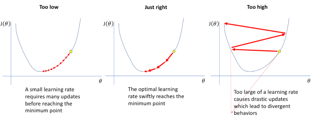
- “It is a scale of how big your model should update it’s weights and biases after every step. Normally, at the beginning of the training, you would want to gradients to update fast. Then, after a certain amount of step, you should decrease the learning rate.” (source)
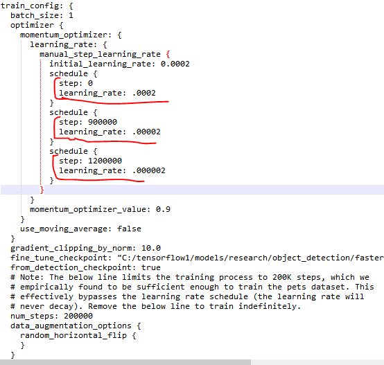
- In the training process of a machine learning model, it is common to start with a relatively large learning rate to allow the model to quickly explore different areas of the parameter space and find a set of weights that yield reasonably good performance. This initial phase helps the model to escape from poor local optima.
- As the training progresses, the learning rate is typically reduced gradually or dynamically. This allows the model to make smaller adjustments to the weights, fine-tuning them to improve accuracy and converge towards the optimal solution. The smaller learning rate helps to make smaller, more precise updates and avoid overshooting the optimal weights.
- Constant learning rate:
- Constant learning rate involves using a fixed learning rate throughout the entire training process.
- This approach is commonly used when the dataset is relatively small and the learning problem is relatively simple.
- It can also be effective when the training data is consistent and the model is not prone to getting stuck in local optima.
- Constant learning rate is straightforward to implement and may converge quickly if the learning rate is appropriately set.
- Cosine decay:
- Cosine decay involves gradually reducing the learning rate over time following a cosine function.
- This approach is often employed when training deep neural networks or complex models with a large amount of data.
- Cosine decay helps the model to converge more smoothly by gradually reducing the learning rate.
- It allows the model to make smaller and more refined weight updates as the training progresses, which can improve the accuracy and generalization of the model.
- The choice of cosine decay can also be motivated by the desire to avoid overshooting the optimal solution and achieving better convergence.
- One such learning rate scheduling strategy can be, starting with an increased learning rate, followed by a constant hold, and then applying cosine decay, can be a valid approach in certain scenarios. Here’s a breakdown of each stage:
- Increasing the learning rate: Starting with a relatively high learning rate can help the model make larger initial weight updates and explore the parameter space more quickly. This can be beneficial in the early stages of training when the model needs to find a reasonable solution faster.
- Constant hold: After the initial increase, you may choose to keep the learning rate constant for a certain number of epochs or until a specific condition is met. This allows the model to stabilize and fine-tune its performance based on the knowledge gained during the initial high learning rate phase.
- Cosine decay: Once the model has reached a relatively stable state, applying cosine decay gradually reduces the learning rate over time. This schedule helps the model make smaller and more precise weight updates, allowing it to converge towards an optimal solution more smoothly. The cosine decay can prevent overshooting and improve the model’s accuracy and generalization.
- When fine-tuning a pre-trained model, it is often recommended to lower the learning rate compared to the initial training phase. Fine-tuning involves taking a pre-trained model and further training it on a new task or dataset. Lowering the learning rate during this stage helps to ensure that the model does not make drastic updates to its parameters and instead focuses on refining its learned representations to better fit the new data.
- Use techniques such as learning rate schedules, grid search, or adaptive learning rate methods to find an optimal learning rate.
- Pros: An appropriate learning rate helps the model converge faster and achieve better performance.
- Cons: Choosing an incorrect learning rate can lead to slow convergence, instability, or suboptimal results.
How many attention layers do I need if I leverage a Transformer?
- The original Transformer model, as introduced in the “Attention is All You Need” paper by Vaswani et al., consists of six identical layers for both the encoder and decoder. However, this is not a strict rule, and the number of layers can be adjusted based on the requirements of the task.
- In general, increasing the number of attention layers can enhance the model’s capacity to capture complex patterns and dependencies in the data. However, a higher number of layers also increases computational requirements and may lead to overfitting if the dataset is not sufficiently large.
- It is common to start with a smaller number of attention layers, such as 4-6 layers, and then incrementally increase or decrease the number based on empirical evaluation and performance on validation data. Ultimately, the optimal number of attention layers is determined through experimentation and careful tuning specific to the task at hand.
Params, Weights, and Features
- Features:
- Features are the individual measurable characteristics or attributes that describe the entities in a given problem. In a recommendation system, features represent properties or characteristics of users and items (movies in this case). Features can include genre, director, release year, actors, user demographics, previous movie ratings, and so on. These features provide quantitative or categorical information that helps to represent and differentiate the entities being considered.
- Weights:
- Weights are parameters associated with each feature in a machine learning model. These weights determine the relative importance or contribution of each feature towards the final prediction or output of the model. In a recommendation system, the weights associated with features represent the significance or influence of those features in determining user preferences or item recommendations.
- During the training process, the model learns these weights by adjusting their values based on the input data and the desired output. The objective is to find the optimal combination of feature weights that minimize the prediction error or loss function.
- In a recommendation system using collaborative filtering, the weights associated with user features indicate how much importance is given to each feature in capturing user preferences. Similarly, the weights associated with movie features indicate the significance of each feature in representing the characteristics of movies. By learning and updating these weights, the model can capture the relationships and patterns between features and make accurate predictions or recommendations.
- Assume we have the following simplified movie recommendation model with the following parameters:
- User-Feature Matrix Parameters:
- Each user is represented by a feature vector capturing their preferences across different movie genres (comedy, action, romance).
- For example, let’s say we have User 1 with the following feature vector: [0.8, 0.2, 0.6].
- The associated parameters for User 1’s feature vector could be: [1.2, 0.9, 0.6].
- These parameters represent the weights or preferences of User 1 towards comedy, action, and romance genres, respectively.
- Movie-Feature Matrix Parameters:
- Each movie is represented by a feature vector describing its attributes, such as genre, director, and actors.
- Let’s consider a movie, Movie A, with the following feature vector: [0.5, 0.7, 0.9].
- The associated parameters for Movie A’s feature vector could be: [0.9, 0.5, 1.0].
- These parameters represent the weights or importance of each feature for Movie A, such as the significance of genre, director, and actors in determining its characteristics.
- During the training phase, these parameters are learned by adjusting their values to minimize the prediction error or loss. The model updates the parameters based on user ratings or preferences for movies and iteratively refines them to improve the recommendation accuracy.
- Once the parameters are learned, the model uses them to make personalized recommendations. For example, the model may calculate the similarity between User 1’s feature vector and the feature vectors of unseen movies, combining the associated parameters to predict the user’s rating for each movie. Based on these predictions, the model can recommend the top-rated movies to User 1.
Evaluating Model Architecture Effectiveness
-
Evaluation Metrics: Determine the model’s accuracy using evaluation metrics tailored to the specific problem, such as accuracy, precision, recall, F1 score, MSE, or MAE. These metrics should be benchmarked against established baselines or industry norms to understand the model’s relative performance.
-
Training Analysis via Learning Curves: Utilize learning curves to visualize the model’s training progress. These curves should illustrate improvements in performance metrics as training progresses, indicating the model’s learning capability and convergence trends.
-
Generalization through Cross-Validation: Implement cross-validation, like k-fold cross-validation, to verify the model’s ability to generalize to new data. This approach provides a robust performance estimate by averaging results across different data partitions.
-
Diagnosing Overfitting and Underfitting: Monitor for overfitting, where the model excels on training data but fails to generalize, and underfitting, where the model can’t capture data patterns. Diagnostics include analyzing performance metrics and learning curves.
-
Model Complexity Review: Examine whether the model’s complexity is proportional to the problem’s complexity. Seek a sweet spot where the architecture is neither too simple to learn the patterns nor too complex that it becomes inefficient or overfitting.
-
Benchmarking Performance: Contrast the model’s effectiveness with cutting-edge models or benchmarks. This comparison can reveal whether the chosen architecture performs competitively within the field.
-
Field Testing: Assess the model in a real-world scenario to understand its practical performance. Monitoring KPIs and gathering user feedback can shed light on how well the model serves its intended purpose.
-
Balance of Complexity and Interpretability: Appraise the model for both its predictive power and the ease with which its decisions can be understood. In fields where clarity is paramount, the trade-off between accuracy and transparency is critical.
Generate Embeddings
- TF-IDF (Term Frequency-Inverse Document Frequency):
- TF-IDF is a popular technique used for text-based recommender systems. It represents the importance of a term (word) in a document within a corpus. Here’s how it works:
- Corpus Preparation: Collect a corpus of textual data, such as product descriptions, user reviews, or item attributes.
- Text Preprocessing: Clean the text data by removing punctuation, stopwords, and applying techniques like stemming or lemmatization.
- Term Frequency (TF): Calculate the frequency of each term (word) in each document (item) within the corpus. This represents how often a term appears in a document.
- Inverse Document Frequency (IDF): Measure the rarity of each term across the entire corpus. This is done by calculating the logarithm of the inverse of the term’s document frequency (number of documents containing the term divided by the total number of documents).
- TF-IDF Calculation: Multiply the term frequency (TF) with the inverse document frequency (IDF) to obtain the TF-IDF score for each term in each document. This score represents the importance of the term in the document compared to its frequency in the corpus.
- Embedding Representation: Treat each document (item) as a vector, where each dimension corresponds to a term in the corpus. The TF-IDF score of a term in a document becomes the value in the corresponding dimension of the vector. These vectors serve as embeddings for the documents.
- TF (Term Frequency) helps capture the importance of a term within a specific movie description. It indicates how frequently a term appears in the movie’s content and helps identify the prominent themes or topics within the description. High TF values for certain terms suggest their significance in describing the movie.
- However, TF alone may not be sufficient to differentiate between common terms and those that are truly informative or distinctive. This is where IDF (Inverse Document Frequency) comes into play. IDF measures the rarity or uniqueness of a term across the entire movie corpus. It helps identify terms that are less common across movies but hold more discriminative power.
- By combining TF and IDF through the TF-IDF approach, the resulting scores reflect both the local importance of terms within a movie’s description (TF) and the global distinctiveness of those terms across the movie collection (IDF). This allows the recommendation system to highlight terms that are both prominent within a movie and unique compared to other movies, enabling more accurate content-based filtering.
- BM-25
- While both BM25 and TF-IDF are term weighting schemes used in information retrieval and text mining, they have some fundamental differences in how they calculate the importance or relevance of terms in a document.
- Calculation:
- TF-IDF (Term Frequency-Inverse Document Frequency) calculates the weight of a term based on its frequency within a document (TF) and its rarity across the entire document collection (IDF).
- BM25 (Best Match 25) also takes into account the term frequency within a document but uses a more sophisticated scoring function that considers factors like document length, average document length, and term frequency in the entire collection.
- Document Length:
- TF-IDF treats all documents as having equal length and does not explicitly account for differences in document length.
- BM25 incorporates the document length by penalizing the weight of terms based on the document length. Longer documents tend to have higher term frequencies, so BM25 compensates for this effect.
- Term Frequency Saturation:
- TF-IDF can suffer from term frequency saturation, where the importance of a term plateaus after a certain frequency threshold.
- BM25 addresses this issue by using a term frequency saturation function that prevents excessive term weight for high frequencies.
- Word Embeddings:
- Word embeddings capture the semantic meaning of words by representing them as dense, low-dimensional vectors. These embeddings are trained using neural network models, such as Word2Vec, GloVe, or FastText, on large corpora. Here’s a general process:
- Corpus Preparation: Gather a large corpus of text data, such as news articles, social media posts, or web documents.
- Tokenization: Split the text into individual words or subword units, known as tokens.
- Neural Network Training: Train a neural network model, such as Word2Vec, on the corpus. This model learns to predict the context (surrounding words) of a given word or vice versa.
- Embedding Extraction: Extract the learned weights from the trained model for each word. These weights form the word embeddings, where each word is represented by a dense vector.
- Pre-trained Embeddings: Alternatively, you can use pre-trained word embeddings that are trained on large external corpora, such as Google’s Word2Vec or Stanford’s GloVe. These pre-trained embeddings can be directly used in recommender systems without training on a specific corpus.
- Collaborative Filtering Embeddings:
- Collaborative filtering techniques consider user-item interactions to generate embeddings. Two common approaches are:
- Matrix Factorization: Factorize a user-item interaction matrix into lower-dimensional matrices representing user and item embeddings. The latent factors capture the underlying preferences or characteristics of users and items.
- Neural Collaborative Filtering: Utilize neural networks, such as Multi-Layer Perceptrons (MLPs) or Deep Neural Networks (DNNs), to learn user and item embeddings from interaction data. These embeddings can capture complex patterns and non-linear relationships.
- Hybrid Approaches:
- Hybrid recommender systems combine multiple types of embeddings to leverage both content and collaborative information. These embeddings can be concatenated, combined using weighted averages, or passed through additional layers to learn a joint representation.
- The choice of embedding method depends on the nature of the data and the specific goals of the recommender system. It is common to experiment with different approaches and evaluate their performance using metrics like precision, recall, or mean average precision (MAP
import pandas as pd
from scipy.sparse import csr_matrix
from sklearn.decomposition import TruncatedSVD

# Load the movie ratings data
ratings_data = pd.read_csv("ratings.csv")

# Create a sparse user-item matrix
user_item_matrix = ratings_data.pivot(index="user_id", columns="movie_id", values="rating").fillna(0)
sparse_matrix = csr_matrix(user_item_matrix.values)

# Apply Singular Value Decomposition (SVD)
svd = TruncatedSVD(n_components=100)
movie_embeddings = svd.fit_transform(sparse_matrix)

# Print the movie embeddings
print(movie_embeddings)
What are the differences between a model that minimizes squared error and the one that minimizes the absolute error? and in which cases each error metric would be more appropriate?
- Both mean square error (MSE) and mean absolute error (MAE) measures the distances between vectors and express average model prediction in units of the target variable. Both can range from 0 to infinity, the lower they are the better the model.
- The main difference between them is that in MSE the errors are squared before being averaged while in MAE they are not. This means that a large weight will be given to large errors. MSE is useful when large errors in the model are trying to be avoided. This means that outliers affect MSE more than MAE (because large errors have a greater influence than small errors), that is why MAE is more robust to outliers.
- Computation-wise MSE is easier to use as the gradient calculation will be more straightforward than MAE, since MAE requires linear programming to calculate it.
Given a left-skewed distribution that has a median of 60, what conclusions can we draw about the mean and the mode of the data?
- Left skewed distribution means the tail of the distribution is to the left and the tip is to the right. So the mean which tends to be near outliers (very large or small values) will be shifted towards the left or in other words, towards the tail.
- While the mode (which represents the most repeated value) will be near the tip and the median is the middle element independent of the distribution skewness, therefore it will be smaller than the mode and more than the mean.
- Thus,
- Mean < 60
- Mode > 60
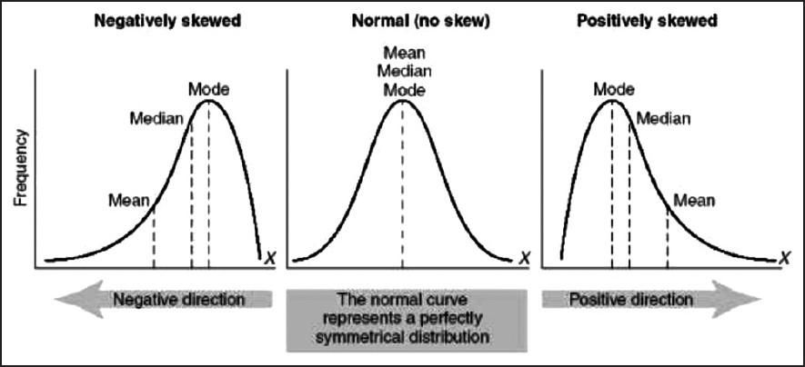
Can you explain the parameter sharing concept in deep learning?
- Parameter sharing is the method of sharing weights by all neurons in a particular feature map. Therefore helps to reduce the number of parameters in the whole system, making it computationally cheap. It basically means that the same parameters will be used to represent different transformations in the system. This basically means the same matrix elements may be updated multiple times during backpropagation from varied gradients. The same set of elements will facilitate transformations at more than one layer instead of those from a single layer as conventional. This is usually done in architectures like Siamese that tend to have parallel trunks trained simultaneously. In that case, using shared weights in a few layers (usually the bottom layers) helps the model converge better. This behavior, as observed, can be attributed to more diverse feature representations learned by the system. Since neurons corresponding to the same features are triggered in varied scenarios. Helps to model to generalize better.
- Note that sometimes the parameter sharing assumption may not make sense. This is especially the case when the input images to a ConvNet have some specific centered structure, where we should expect, for example, that completely different features should be learned on one side of the image than another.
- One practical example is when the input is faces that have been centered in the image. You might expect that different eye-specific or hair-specific features could (and should) be learned in different spatial locations. In that case, it is common to relax the parameter sharing scheme, and instead, simply call the layer a Locally-Connected Layer.
What is the meaning of selection bias and how to avoid it?
-
Sampling bias is the phenomenon that occurs when a research study design fails to collect a representative sample of a target population. This typically occurs because the selection criteria for respondents failed to capture a wide enough sampling frame to represent all viewpoints.
- The cause of sampling bias almost always owes to one of two conditions.
- Poor methodology: In most cases, non-representative samples pop up when researchers set improper parameters for survey research. The most accurate and repeatable sampling method is simple random sampling where a large number of respondents are chosen at random. When researchers stray from random sampling (also called probability sampling), they risk injecting their own selection bias into recruiting respondents.
- Poor execution: Sometimes data researchers craft scientifically sound sampling methods, but their work is undermined when field workers cut corners. By reverting to convenience sampling (where the only people studied are those who are easy to reach) or giving up on reaching non-responders, a field worker can jeopardize the careful methodology set up by data scientists.
- The best way to avoid sampling bias is to stick to probability-based sampling methods. These include simple random sampling, systematic sampling, cluster sampling, and stratified sampling. In these methodologies, respondents are only chosen through processes of random selection—even if they are sometimes sorted into demographic groups along the way.
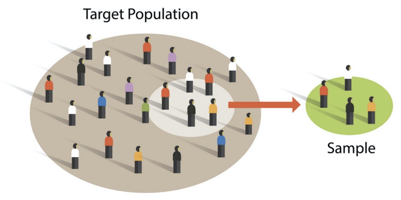
Define the cross-validation process and the motivation behind using it?
-
Cross-validation is a technique used to assess the performance of a learning model in several subsamples of training data. In general, we split the data into train and test sets where we use the training data to train our model and the test data to evaluate the performance of the model on unseen data and validation set for choosing the best hyperparameters. Now, a random split in most cases (for large datasets) is fine. But for smaller datasets, it is susceptible to loss of important information present in the data in which it was not trained. Hence, cross-validation though computationally bit expensive combats this issue.
-
The process of cross-validation is as the following:
- Define \(k\) or the number of folds.
- Randomly shuffle the data into \(k\) equally-sized blocks (folds).
- For each \(i\) in fold (1 to \(k\)), train the data using all the folds except for fold \(i\) and test on the fold \(i\).
- Average the \(k\) validation/test error from the previous step to get an estimate of the error.
- This process aims to accomplish the following:
- Prevent overfitting during training by avoiding training and testing on the same subset of the data points
- Avoid information loss by using a certain subset of the data for validation only. This is important for small datasets.
- Cross-validation is always good to be used for small datasets, and if used for large datasets the computational complexity will increase depending on the number of folds.
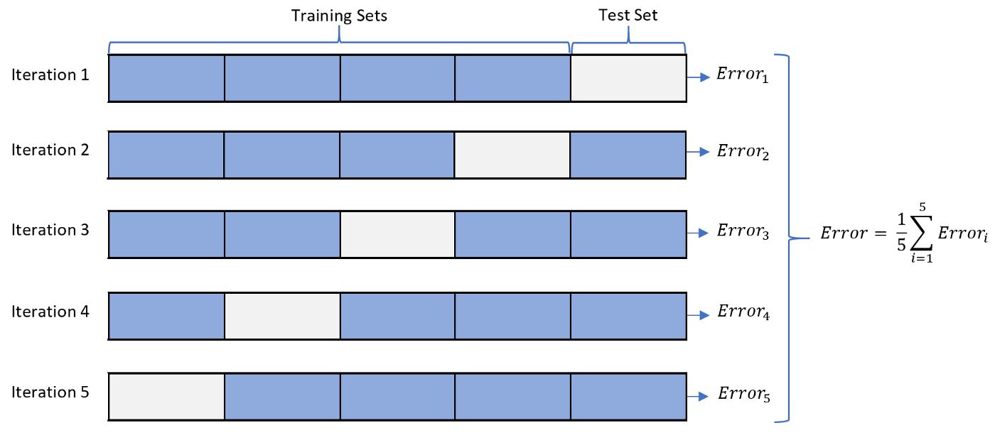
Explain the long-tailed distribution and provide three examples of relevant phenomena that have long tails. Why are they important in classification and regression problems?
- A long-tailed distribution is a type of heavy-tailed distribution that has a tail (or tails) that drop off gradually and asymptotically.
- Three examples of relevant phenomena that have long tails:
- Frequencies of languages spoken
- Population of cities
- Pageviews of articles
- All of these follow something close to the 80-20 rule: 80% of outcomes (or outputs) result from 20% of all causes (or inputs) for any given event. This 20% forms the long tail in the distribution.
- It’s important to be mindful of long-tailed distributions in classification and regression problems because the least frequently occurring values make up the majority of the population. This can ultimately change the way that you deal with outliers, and it also conflicts with some machine learning techniques with the assumption that the data is normally distributed.
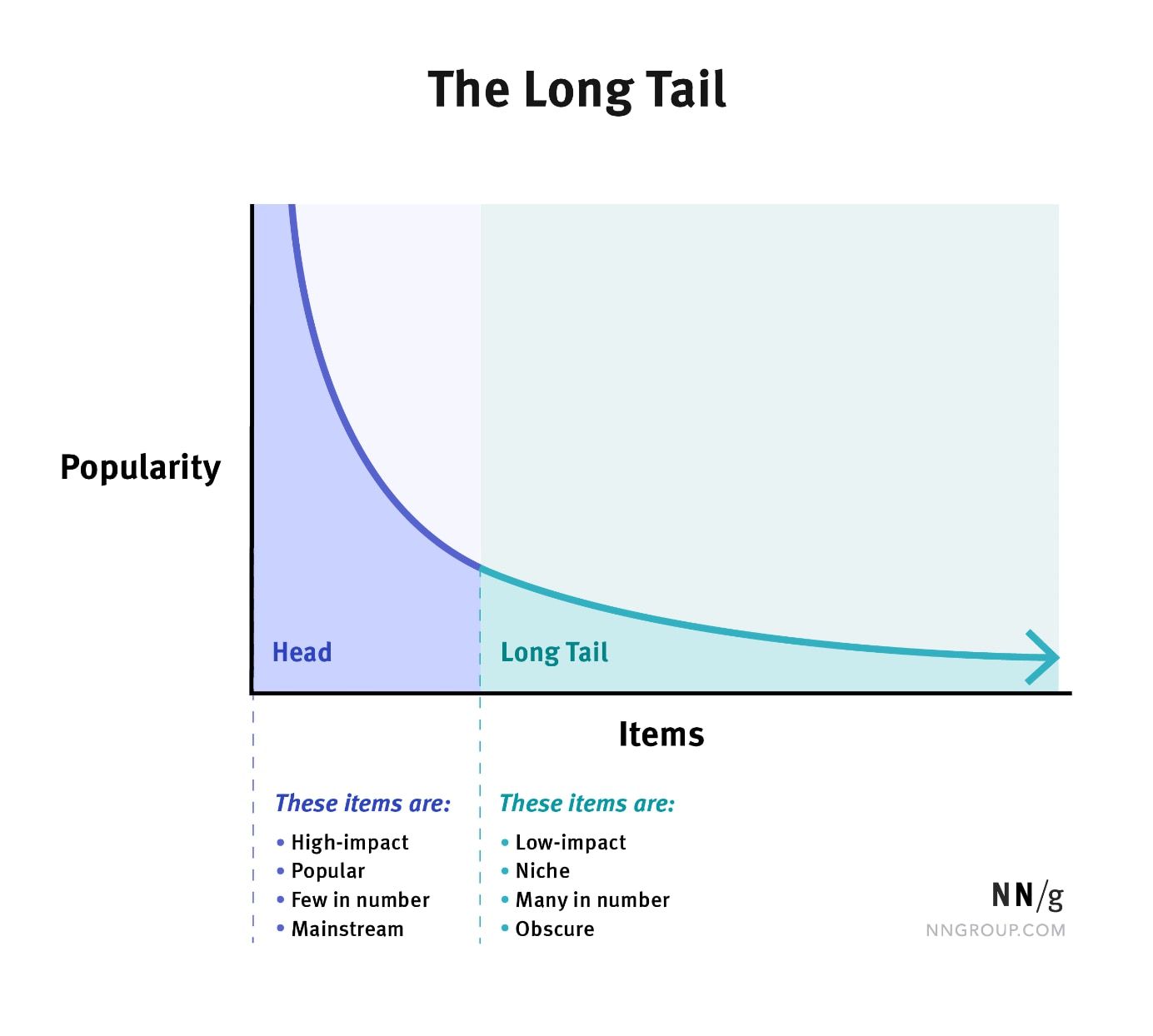
You are building a binary classifier and found that the data is imbalanced, what should you do to handle this situation?
- If there is a data imbalance there are several measures we can take to train a fairer binary classifier:
- Pre-Processing:
- Check whether you can get more data or not.
- Use sampling techniques (Up-sample minority class, downsample majority class, can take the hybrid approach as well). We can also use data augmentation to add more data points for the minority class but with little deviations/changes leading to new data points which are similar to the ones they are derived from. The most common/popular technique is SMOTE (Synthetic Minority Oversampling technique)
- Suppression: Though not recommended, we can drop off some features directly responsible for the imbalance.
- Learning Fair Representation: Projecting the training examples to a subspace or plane minimizes the data imbalance.
- Re-Weighting: We can assign some weights to each training example to reduce the imbalance in the data.
- In-Processing:
- Regularizaion: We can add score terms that measure the data imbalance in the loss function and therefore minimizing the loss function will also minimize the degree of imbalance with respect to the score chosen which also indirectly minimizes other metrics which measure the degree of data imbalance.
- Adversarial Debiasing: Here we use the adversarial notion to train the model where the discriminator tries to detect if there are signs of data imbalance in the predicted data by the generator and hence the generator learns to generate data that is less prone to imbalance.
- Post-Processing:
- Odds-Equalization: Here we try to equalize the odds for the classes w.r.t. the data is imbalanced for correct imbalance in the trained model. Usually, the F1 score is a good choice, if both precision and recall scores are important
- Choose appropriate performance metrics. For example, accuracy is not a correct metric to use when classes are imbalanced. Instead, use precision, recall, F1 score, and ROC curve.
- Pre-Processing:
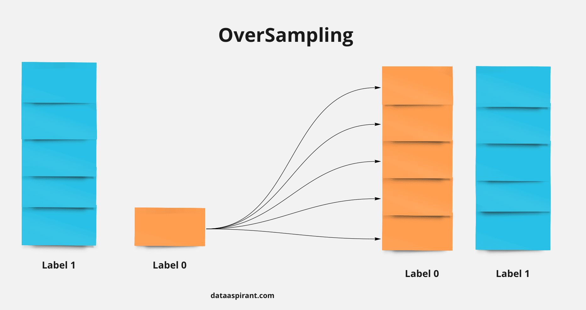
What to do with imbalance class
- Dealing with imbalanced classes is a common challenge in machine learning, where the number of instances in one class significantly outweighs the number of instances in another class. This issue can negatively impact the performance and accuracy of the machine learning model, as it tends to favor the majority class.
- Some common issues associated with imbalanced classes are:
- Biased Model: The model may favor the majority class, leading to low recall or sensitivity for the minority class, which can be problematic in scenarios where detecting the minority class is critical.
- Poor Generalization: Imbalanced data can hinder the model’s ability to generalize well to unseen data, as it may not adequately capture the underlying patterns of the minority class.
- Evaluation Metrics: Traditional accuracy may not be an appropriate evaluation metric, as a model predicting only the majority class can still achieve high accuracy in an imbalanced setting. Alternative metrics like precision, recall, F1-score, and area under the Receiver Operating Characteristic (ROC) curve are more suitable.
- Resampling Techniques:
- Undersampling: Randomly remove samples from the majority class to balance the class distribution.
- Oversampling: Create synthetic samples in the minority class to increase its representation.
- SMOTE (Synthetic Minority Over-sampling Technique): Generate synthetic samples by interpolating between existing minority class samples.
- ADASYN (Adaptive Synthetic Sampling): Similar to SMOTE, but gives more emphasis to difficult-to-learn minority samples.
- Class Weighting:
- Assign higher weights to the minority class during model training to penalize misclassifications and encourage better classification of the minority class.
- Ensemble Methods:
- Combine multiple models trained on different subsets of the data or using different algorithms to improve overall performance and handle class imbalance.
- Anomaly Detection:
- Treat the minority class as an anomaly and use techniques such as One-Class SVM or Isolation Forest to detect and classify instances of the minority class.
- Collect More Data:
- If possible, collect additional data for the minority class to improve its representation and address the class imbalance problem.
- Evaluation Metrics:
- Instead of solely relying on accuracy, consider using evaluation metrics that are robust to imbalanced classes, such as precision, recall, F1-score, area under the ROC curve (AUC-ROC), or precision-recall curve.
It’s important to note that the choice of approach depends on the specific problem, dataset, and the underlying reasons for class imbalance. Experimentation and careful evaluation of different techniques are necessary to find the most effective solution.
By employing these techniques and adapting them to the specific problem at hand, we can mitigate the impact of imbalanced classes and improve the overall performance and fairness of our machine learning models.
What is the Vanishing Gradient Problem and how do you fix it?
- The vanishing gradient problem is encountered in artificial neural networks with gradient-based learning methods and backpropagation. In these learning methods, each of the weights of the neural network receives an update proportional to the partial derivative of the error function with respect to the current weight in each iteration of training. Sometimes when gradients become vanishingly small, this prevents the weight to change value.
- When the neural network has many hidden layers, the gradients in the earlier layers will become very low as we multiply the derivatives of each layer. As a result, learning in the earlier layers becomes very slow. This can cause the network to stop learning. This problem of vanishing gradients happens when training neural networks with many layers because the gradient diminishes dramatically as it propagates backward through the network.
- Some ways to fix it are:
- Use skip/residual connections.
- Using ReLU or Leaky ReLU over sigmoid and tanh activation functions.
- Use models that help propagate gradients to earlier time steps such as GRUs and LSTMs.
What are Residual Networks? How do they help with vanishing gradients?
- Here is a concept that you should know whether you are trying to get a job in AI or you want to improve your knowledge of AI: residual networks.
How do you run a deep learning model efficiently on-device?
- Let’s take the example of LLaMA, a ChatGPT-like LLM by Meta.
- You can run one of the latest LLMs if you have a computer with 4Gb of RAM.
- The model is implemented in C++ (with Python wrappers) and uses several optimization techniques:
- Quantization
- Quantization represents the weights of the model in a low-precision data type like 4-bit integer (INT4) instead of the usual 32-bit floating precision (FP32).
- For example, the smallest LLaMA model has 7B parameters.
- The original model uses 13GB of RAM, while the optimized model uses 3.9GB.
- Faster weight loading
- Another optimization is to load the model weights using
mmap()instead of standard C++ I/O. - That enabled to load LLaMA 100x faster using half as much memory.
mmap()maps the read-only weights usingMAP_SHARED, which is the same technique that’s traditionally used for loading executable software.
- Another optimization is to load the model weights using
- Quantization
Evaluating Model Architecture Effectiveness
-
Evaluation Metrics: Determine the model’s accuracy using evaluation metrics tailored to the specific problem, such as accuracy, precision, recall, F1 score, MSE, or MAE. These metrics should be benchmarked against established baselines or industry norms to understand the model’s relative performance.
-
Training Analysis via Learning Curves: Utilize learning curves to visualize the model’s training progress. These curves should illustrate improvements in performance metrics as training progresses, indicating the model’s learning capability and convergence trends.
-
Generalization through Cross-Validation: Implement cross-validation, like k-fold cross-validation, to verify the model’s ability to generalize to new data. This approach provides a robust performance estimate by averaging results across different data partitions.
-
Diagnosing Overfitting and Underfitting: Monitor for overfitting, where the model excels on training data but fails to generalize, and underfitting, where the model can’t capture data patterns. Diagnostics include analyzing performance metrics and learning curves.
-
Model Complexity Review: Examine whether the model’s complexity is proportional to the problem’s complexity. Seek a sweet spot where the architecture is neither too simple to learn the patterns nor too complex that it becomes inefficient or overfitting.
-
Benchmarking Performance: Contrast the model’s effectiveness with cutting-edge models or benchmarks. This comparison can reveal whether the chosen architecture performs competitively within the field.
-
Field Testing: Assess the model in a real-world scenario to understand its practical performance. Monitoring KPIs and gathering user feedback can shed light on how well the model serves its intended purpose.
-
Balance of Complexity and Interpretability: Appraise the model for both its predictive power and the ease with which its decisions can be understood. In fields where clarity is paramount, the trade-off between accuracy and transparency is critical.
Underfitting
- Underfitting occurs when a model is too simple and fails to learn essential patterns in the training data. It results in poor performance on both the training data and new, unseen data. Underfitting can be identified by analyzing the learning curve, where the model’s performance remains consistently low.
- To avoid underfitting, the following techniques can be employed:
- Increase the complexity of the model.
- Increase the number of input features.
- Allow the model to train for a longer duration. 1. Enhance Model Complexity: Switch to more complex models or architectures that can capture intricate patterns, e.g., moving from a linear model to a polynomial or non-linear model. 2. Incorporate More Features: If relevant, bring in additional input features that might help the model understand the data better. 3. Prolonged Training: Increase the number of epochs or training iterations, ensuring that the model has adequate time to learn. 4. Feature Engineering: Create new features from existing ones that might better capture the underlying patterns. 5. Hybrid Models: Combine two or more algorithms to take advantage of their combined strengths. 6. Tweak Model Parameters: Adjusting hyperparameters can sometimes help, like increasing the depth of decision trees. 7. Use Advanced Optimization Techniques: Employ techniques like gradient boost to optimize and fine-tune the model. 8. Remove Noise: Clean the dataset to remove any noise or irrelevant data, ensuring that the model has a clear signal to learn from.
Overfitting
- Overfitting happens when a model is overly complex and tries to memorize the training data instead of learning underlying patterns. It performs well on the training data but fails to generalize to new, unseen data. Overfitting can be detected through the learning curve, which shows a significant gap between the performance on the training set and the performance on the validation or test set.
- To avoid overfitting, the following techniques can be employed:
- Increase the number of training examples.
- Use techniques such as feature selection, creating ensembles, dimensionality reduction, regularization, cross-validation, and early stopping.
- Utilize neural network-specific techniques like dropout, L1 and L2 regularization, early stopping, data augmentation, and noise regularization. 1. Increase Dataset Size: Add more training examples, which can be achieved organically or through techniques like bootstrapping or data augmentation. 2. Cross-Validation: Use techniques like k-fold cross-validation to get a more accurate estimate of model performance. 3. Regularization: Apply L1 (Lasso) or L2 (Ridge) regularization to penalize certain model parameters if they’re likely causing overfitting. 4. Prune the Model: For decision trees, prune branches that add little predictive power. For neural networks, consider dropout layers. 5. Feature Selection: Choose a subset of all available features to reduce dimensionality and prevent the model from relying on noise. 6. Early Stopping: In iterative models like neural networks, halt training when performance on a validation set stops improving and where the model’s performance on a held-out validation dataset does not get better, and may even begin to get worse, over successive training iterations or epochs.. 7. Dimensionality Reduction: Techniques like Principal Component Analysis (PCA) or t-SNE can help in reducing the number of features. 8. Ensemble Methods: Use techniques like bagging or boosting to average out the predictions of multiple models, which can help in reducing overfitting.
How do you avoid overfitting? Try one (or more) of the following:
-
Training with more data, which makes the signal stronger and clearer, and can enable the model to detect the signal better. One way to do this is to use #dataaugmentation strategies
-
Reducing the number of features in order to avoid the curse of dimensionality (which occurs when the amount of data is too low to support highly-dimensional models), which is a common cause for overfitting
-
Using cross-validation. This technique works because the model is unlikely to make the same mistake on multiple different samples, and hence, errors will be evened out
-
Using early stopping to end the training process before the model starts learning the noise
-
Using regularization and minimizing the adjusted loss function. Regularization works because it discourages learning a model that’s overly complex or flexible
-
Using ensemble learning, which ensures that the weaknesses of a model are compensated by the other ones
Data Drift
- Data drift occurs when there is a change in the statistical properties of the input data for a model over time, causing the data the model was trained on to no longer be representative of the current environment. This discrepancy can lead to a drop in model performance and prediction accuracy.
Fine-Tuning in Deep Learning
Theoretical Overview
- Fine-tuning refers to taking a pretrained model and adapting it to a new task by updating some or all of its weights using new data.
- It is often used when training from scratch is too expensive or insufficient data is available.
Types of Fine-Tuning
- Full Fine-Tuning
- All model weights are updated.
- High flexibility but requires significant compute and memory.
- Best for when the target task is significantly different from the pretraining task.
- Example Use Cases: Adapting a pretrained BERT model for a completely different NLP domain.
- Parameter-Efficient Fine-Tuning (PEFT)
- Updates only a small subset of parameters while freezing most layers.
- Saves memory and speeds up training, making it ideal for large models (e.g., LLaMA, GPT).
- Popular PEFT Methods:
- LoRA (Low-Rank Adaptation): Injects small trainable matrices into transformer layers.
- Adapters: Introduces lightweight layers between existing layers.
- Prefix-Tuning: Learns a small set of task-specific parameters prepended to input embeddings.
- Example Use Cases: Personalizing GPT-3.5, LLaMA, Stable Diffusion, etc.
Libraries for Fine-Tuning
✅ Hugging Face transformers – NLP models (BERT, GPT, T5)
✅ peft (Hugging Face) – LoRA, Adapters, P-Tuning
✅ TensorFlow/Keras tf.keras.Model.fit() – Simple fine-tuning in DL
✅ PyTorch torch.nn.Module – Fully custom fine-tuning
Code Examples for Each Approach
1️⃣ Full Fine-Tuning (Hugging Face Transformers)
from transformers import AutoModelForSequenceClassification, AutoTokenizer, Trainer, TrainingArguments

model_name = "bert-base-uncased"
model = AutoModelForSequenceClassification.from_pretrained(model_name, num_labels=2)
tokenizer = AutoTokenizer.from_pretrained(model_name)

training_args = TrainingArguments(output_dir="./results", num_train_epochs=3, per_device_train_batch_size=8)
trainer = Trainer(model=model, args=training_args, train_dataset=train_data, eval_dataset=eval_data)
trainer.train()
2️⃣ LoRA (PEFT) – Efficient Fine-Tuning
from transformers import AutoModelForCausalLM
from peft import LoraConfig, get_peft_model

model = AutoModelForCausalLM.from_pretrained("meta-llama/Llama-2-7b", device_map="auto")

lora_config = LoraConfig(r=8, lora_alpha=16, target_modules=["q_proj", "v_proj"], lora_dropout=0.1)
model = get_peft_model(model, lora_config)
model.train()  # Now, only the LoRA-adapted layers will be trained
- Fine-tuning adapts pretrained models to new tasks with different levels of compute efficiency.
- Full fine-tuning is powerful but expensive.
- PEFT (LoRA, Adapters, Prefix-Tuning) is optimal for large models like GPT, LLaMA.
- Feature extraction is a quick method for similar-task adaptation.
Strategies to Manage Data and Semantic Shift
- Organizations must adopt proactive measures to handle data and semantic shift effectively:
-
Continuous Data Monitoring: This involves setting up a system to continually observe the input data for changes in distribution. It uses statistical analysis, visualizations, or automated monitoring tools to spot deviations.
-
Data Preprocessing and Feature Engineering: With new data, preprocessing and feature engineering ensure the model can still understand and process the information correctly. This might mean adjusting or expanding preprocessing routines to accommodate new data variations.
-
Model Retraining and Updating: If data drift is significant, retraining the model with fresh data might be necessary. Techniques like transfer learning can also be utilized to adjust pre-trained models to new data contexts.
-
Ensemble Modeling: Using a collection of models with different data or architectures can help make the system more robust against data drift, as it relies on collective decision-making from various models.
-
Feedback Loops and User Feedback: Establish channels for user or expert feedback to identify when the model’s outputs are not aligning with real-world results. This insight can be crucial in recognizing data or semantic shifts.
-
Human-in-the-Loop: Integrating human judgment can help manage uncertain cases, especially when data drift may impact model predictions.
-
Model Audits and Performance Evaluations: Periodic reviews of the model’s predictions against real outcomes can identify performance issues early.
-
Data Governance and Documentation: Proper tracking and recording of any changes in data processing, sources, and model updates are vital for transparency and managing drift over time.
Detecting Data Drift
There are several techniques for detecting data drift:
-
Statistical Measures: Regularly compare statistical metrics like mean or variance to flag changes in data distributions.
-
Drift Detection Algorithms: Utilize algorithms such as the Drift Detection Method (DDM) or the Page-Hinkley test, which are designed to detect changes in data distribution.
-
Hypothesis Testing: Perform statistical tests, such as the Kolmogorov-Smirnov or chi-square tests, to check if there are significant differences in distributions over time.
-
Monitoring Model Performance: Keep an eye on model performance metrics like accuracy or precision. Deterioration may indicate data drift.
-
Model Prediction Drift Detection: Look at shifts in the model’s predictions compared to new data or ground truth to identify drift.
Continuous Training & Testing: Beyond Data Drift
Data Validation: It’s vital to ensure the quality of incoming data:
-
Schema Validation: Verify that data schemas match expected formats to prevent downstream issues.
-
Monitoring for Data Drift: Stay vigilant for shifts in data distributions that could compromise model performance.
Model Validation: Before deploying a model, validate:
-
Performance: Test your model against key metrics to ensure it meets predefined thresholds.
-
Versioning and Metadata: Keep track of model versions and metadata, tools like neptune.ai can be helpful.
-
Security: Be aware of potential adversarial attacks, particularly for models with significant decision-making roles.
-
Infrastructure: Ensure your model’s infrastructure is compatible with the prediction service API before deployment.
What is Continuous Training?
Continuous training is the process of persistently retraining machine learning models to adapt to new data or changes in the underlying data distribution before redeployment. The reasons for continuous training include:
-
Model Decay: Models can become less accurate over time due to changes in the real world and user behavior.
-
Covariate Shift: When real-world data deviates from the training data, it can lead to a model’s predictions becoming less reliable.
-
Concept Drift: This is when the relationship between input data and the target variable changes over time, necessitating updates to the model to maintain its accuracy.
Monitoring and Addressing Drift
-
Data Drift Monitoring: Use advanced MLOps tools to continuously review your data, such as the JS-Divergence algorithm or platforms like Fiddler AI, which can provide real-time insights.
-
Concept Drift: Recognize when the model’s understanding of the target variable changes and update the model accordingly to reflect these new patterns.
-
By implementing these strategies and maintaining vigilance for drift, organizations can ensure their AI systems remain effective and accurate over time.
Pretraining vs. Continued Pretraining of Large Language Models (LLMs)
1️⃣ Pretraining vs. Continued Pretraining: Key Differences
- Pretraining trains an LLM from scratch using self-supervised learning (e.g., next-token prediction, masked language modeling) on massive datasets (Common Crawl, Wikipedia, BooksCorpus). This phase requires trillions of tokens and massive compute power (GPUs/TPUs).
- Continued Pretraining further trains an existing LLM on a domain-specific corpus (e.g., legal, medical, financial texts). This specializes the model while leveraging existing general knowledge, reducing compute needs compared to pretraining from scratch.
- Pretraining requires trillions of tokens across diverse data, while continued pretraining focuses on smaller, high-quality datasets (millions to billions of tokens).
- Pretraining is necessary for foundation models (GPT, LLaMA, T5), whereas continued pretraining helps adapt general models to niche domains (e.g., BioGPT for biomedical text).
2️⃣ System-Level Optimizations for Large-Scale Pretraining
✅ Distributed Training (FSDP, ZeRO, DeepSpeed, Megatron-LM)
- Library:
torch.distributed,transformers,deepspeed,Megatron-LM - Fully Sharded Data Parallelism (FSDP) eliminates redundant copies of model states across GPUs.
- Zero Redundancy Optimizer (ZeRO, DeepSpeed) partitions optimizer states, gradients, and parameters to enable training on memory-constrained hardware.
- Tensor Parallelism (
Megatron-LM) splits model layers across GPUs to reduce memory load per device and increase scalability across clusters. - Pipeline Parallelism (
torch.distributed.pipeline) keeps GPUs active by splitting computations across layers running on different devices.
✅ Asynchronous Data Loading & Prefetching
- Library:
torch.utils.data,datasets,TensorFlow data API - Avoids training stalls by keeping GPUs constantly fed with new batches, preventing I/O bottlenecks.
- Uses multi-threaded data loading (
num_workers,prefetch_factor) to maximize throughput.
✅ RDMA & High-Speed Networking for Multi-GPU/TPU Training
- Library:
NCCL,InfiniBand,GPUDirect RDMA,XLA - Uses InfiniBand or NVLink for low-latency GPU-GPU communication, preventing bottlenecks in distributed training.
- NVIDIA GPUDirect RDMA allows direct data transfers between GPUs without involving the CPU, reducing transfer latency.
- TPU Pods (
jax,XLA) are optimized for fast multi-node training using Google’s high-speed TPU interconnects.
3️⃣ Memory & Compute Optimizations for Efficient Pretraining
✅ Flash Attention for Reducing Memory Usage in Transformers
- Library:
flash-attn,xformers,transformers - Recomputes attention matrices on-the-fly instead of storing them, significantly lowering memory usage.
- Optimized for A100, H100, and TPU hardware accelerators.
✅ Gradient Checkpointing to Reduce Memory Overhead
- Library:
torch.utils.checkpoint,deepspeed - Saves GPU memory by recomputing activations during the backward pass instead of storing them.
- Helps train larger models on memory-limited hardware.
✅ Mixed Precision Training (FP16/BF16) for Faster Computation
- Library:
torch.autocast,transformers,TensorFlow mixed precision - Uses lower precision (FP16/BF16) to speed up training while reducing memory usage.
- BF16 is more stable on NVIDIA A100, H100, and TPU hardware than FP16.
✅ Gradient Accumulation for Large Batch Sizes on Small GPUs
- Library:
transformers.Trainer,torch.optim - Simulates large-batch training by accumulating gradients over multiple steps before performing a weight update.
- Allows training on GPUs with limited memory while still benefiting from large effective batch sizes.
✅ Activation Offloading & CPU/GPU Memory Swapping
- Library:
DeepSpeed Offload,torch.cuda.memory_allocated,Ray Serve - Moves activations to CPU memory when not in use, freeing up GPU memory for larger batch sizes.
- DeepSpeed Offload optimizes state storage across GPU/CPU memory hierarchies.
4️⃣ Data Efficiency & Tokenization Strategies
✅ Highly Compressed Tokenization (BPE, SentencePiece, UnigramLM)
- Library:
sentencepiece,tiktoken,transformers - Uses subword tokenization to reduce sequence length and speed up training.
- Tiktoken (used in OpenAI’s GPT models) is optimized for fast tokenization.
✅ Dataset Deduplication to Remove Redundant Text
- Library:
text-dedup,lm-data-cleaning,BigScience-data-tools - Removes duplicate content (e.g., books copied across datasets) to prevent overfitting and redundancy.
✅ Progressive Training (Curriculum Learning)
- Library:
torch.utils.data,datasets,Curriculum Learning PyTorch - Starts with simpler examples first, then progressively introduces harder examples, improving convergence speed.
✅ Efficient Data Shuffling & Batching
- Library:
torch.data.DataLoader,huggingface datasets,TensorFlow data API - Prevents stale gradients by ensuring batches contain diverse linguistic structures and topics rather than consecutive text blocks.
5️⃣ Hardware & Cluster Optimization for Pretraining
✅ High-Bandwidth Memory (HBM) & Large VRAM GPUs
- Library:
torch.cuda,tensorflow.device_lib - NVIDIA A100, H100, TPUv4 use HBM for faster model inference and training.
- Enables larger context windows without degrading performance.
✅ Cloud Compute Optimization (Spot Instances & Auto-Scaling)
- Library:
AWS Sagemaker,Vertex AI,Lambda Labs,SkyPilot - Uses spot instances for cost reduction, requiring robust checkpointing mechanisms to avoid losing progress.
- Deploys auto-scaling to efficiently allocate compute resources based on workload demand.
✅ Energy-Efficient Sparse Training (Mixture of Experts, MoE, Pruning)
- Library:
torch.sparse,MoE-transformers,tutel - Mixture of Experts (MoE) models activate only a subset of parameters per forward pass, reducing compute costs while maintaining accuracy.
- Sparse training techniques prune unnecessary weights to lower FLOPs, improving efficiency.
Describe learning rate schedule/annealing.
- An optimizer is typically used with a learning rate schedule that involves a short warmup phase, a constant hold phase and an exponential decay phase. The decay/annealing is typically done using a cosine learning rate schedule over a number of cycles (Loshchilov & Hutter, 2016).
Explain mean/average in terms of attention.
- Averaging is equivalent to uniform attention.
What is convergence in k-means clustering?
- In case of \(k\)-means clustering, the word convergence means the algorithm has successfully completed clustering or grouping of data points in \(k\) number of clusters. The algorithm determines that it has grouped/clustered the data points into correct clusters if the centroids (\(k\) values) in the last two consequent iterations are same then the algorithm is said to have converged. However, in practice, people often use a less strict criteria for convergence, for e.g., the difference in the values of last two iterations needs to be less than a low threshold.
List some debug steps/reasons for your ML model underperforming on the test data.
- Insufficient quantity of training data: Machine learning algorithms need a large amount of data to be able to learn the underlying statistics from the data and work properly. Even for simple problems, the models will typically need thousands of examples.
- Nonrepresentative training data: In order for the model to generalize well, your training data should be representative of what is expected to be seen in the production. If the training data is nonrepresentative of the production data or is different this is known as data mismatch.
- Poor quality data: Since the learning models will use the data to learn the underlying pattern and statistics from it. It is critical that the data are rich in information and be of good quality. Having training data that are full of outliers, errors, noise, and missing data will decrease the ability of the model to learn from data, and then the model will act poorly on new data.
- Irrelevant features: As the famous quote says “garbage in, garbage out”. Your machine learning model will be only able to learn if the data contains relevant features and not too many irrelevant features.
- Overfitting the training data: Overfitting happens when the model is too complex relative to the size of the data and its quality, which will result in learning more about the pattern in the noise of the data or very specific patterns in the data which the model will not be able to generalize for new instances.
- Underfitting the training data: Underfitting is the opposite of overfitting, the model is too simple to learn any of the patterns in the training data. This could be known when the training error is large and also the validation and test error is large.
Common Errors and how to solve them
Not performing one-hot encoding when using categorical_crossentropy
- When utilizing the categorical_crossentropy loss function, it is essential to apply one-hot encoding to scalar value labels. Failure to do so will result in an error. The error arises because the categorical_crossentropy function expects one-hot encoded labels as input.
- To avoid this error, you can take the following measures:
- Use the sparse_categorical_crossentropy loss function instead of categorical_crossentropy. This function does not require one-hot encoding.
- Perform one-hot encoding on the labels and continue using the categorical_crossentropy loss function. One-hot encoding transforms scalar labels into n-element vectors, where n represents the number of classes. The to_categorical() function can be employed for this purpose.
- By adhering to these guidelines and ensuring proper one-hot encoding, you can effectively prevent errors and employ the categorical_crossentropy loss function accurately in your deep learning models.
Small dataset for complex algorithms
- Deep learning algorithms, such as neural networks, are primarily designed to excel when working with large datasets comprising millions or thousands of millions of training instances. In the case of small datasets, their performance is considerably limited.
- In fact, there are instances where deep learning algorithms perform even worse than conventional machine learning algorithms when applied to small datasets.
Failure to detect outliers in data
- Outliers are often present in real-world datasets, representing data points that deviate significantly from the majority of other data points. These outliers can be visually identified when plotting the data, as they appear distinctly separate from the rest.
- Methods for outlier detection:
- Z-Score or Standard Deviation Method: This method calculates the z-score for each data point based on its deviation from the mean and standard deviation of the dataset. Points with a z-score above a certain threshold (e.g., 3) are considered outliers.
- Several techniques can be employed to detect outliers, including:
- IQR-based detection
- Elliptic envelope
- Isolation forest
- One-class SVM
- Local outlier factor (LOF)
- Handling outliers:
- When dealing with outliers, it is crucial to carefully consider their significance. Simply removing outliers without understanding their underlying story is not recommended. If an outlier carries valuable information relevant to the problem at hand, it should be retained and accounted for in subsequent analysis. However, outliers resulting from data collection errors can be safely removed. Neglecting to address unnecessary outliers can introduce bias to the model and potentially lead to the omission of important patterns within the data.
Failure to verify model assumptions
- When constructing models, we often work under specific assumptions. These assumptions serve as the foundation for accurate predictions, provided they are not violated. Therefore, it is crucial to validate the underlying assumptions once the model is built.
- Examples of validating model assumptions:
- Normality assumption in linear regression: One assumption is that the residuals (the differences between observed and predicted values) in a linear regression model follow a normal distribution with a mean of zero and a fixed standard deviation. To verify this, we can create a histogram of the residuals and ensure they approximate a normal distribution. Additionally, calculating the mean of the residuals and confirming its proximity to zero reinforces this assumption.
- Histogram depicting the distribution of residuals (Image by author)
- Independence assumption in linear regression: Another assumption is that the residuals in a linear regression model are uncorrelated or independent. We can verify this assumption by generating a residual plot, examining the pattern of the residuals to ensure no systematic correlation exists between them.
Failure to utilize a validation set for hyperparameter tuning
- In the process of hyperparameter tuning, it is essential to employ a distinct dataset known as the validation set, in addition to the training and testing datasets. Utilizing the same training data for hyperparameter tuning can result in data leakage, undermining the model’s ability to generalize to new, unseen data.
- To ensure an effective approach, the training set is utilized for fitting the model parameters, the validation set is dedicated to fine-tuning the model’s hyperparameters, and the test set is employed to evaluate the model’s performance. By adhering to this methodology, we can enhance the model’s overall effectiveness and robustness.
- Using a validation set for hyperparameter tuning is crucial for several reasons:
- Preventing Overfitting: Hyperparameter tuning involves adjusting the settings of the model to optimize its performance. Without a validation set, tuning is performed on the same data used for training, which can lead to overfitting. Overfitting occurs when the model becomes too specific to the training data and performs poorly on new, unseen data. By utilizing a separate validation set, we can assess the model’s performance on unseen data and make more informed decisions during hyperparameter tuning.
- Evaluating Generalization: The primary goal of machine learning is to build models that can generalize well to unseen data. A validation set allows us to evaluate the model’s performance on data it hasn’t encountered during training. By tuning the hyperparameters based on the validation set’s performance, we increase the chances of the model’s ability to generalize and perform well on new data.
- Avoiding Data Leakage: Data leakage refers to situations where information from the test or validation set unintentionally leaks into the training process, leading to overly optimistic performance estimates. If the same data is used for both training and hyperparameter tuning, the model can indirectly “learn” about the validation data and bias the tuning process. By using a separate validation set, we ensure that the tuning process remains independent and unbiased.
Less data for training
- Allocating an adequate amount of data for the training set is crucial for effective model learning and generalization. The following points highlight the importance of allocating a sufficient portion of the dataset for training:
- Enhanced Learning: A larger training set allows the model to access a wider range of examples, enabling it to capture diverse patterns and relationships present in the data. With more data, the model can learn more robust representations and make better predictions. Therefore, it is advisable to allocate a significant portion of the data for training.
- Generalization Improvement: A well-trained model should be capable of performing well on unseen data. By providing a substantial training set, the model has a better chance of learning the underlying patterns that generalize to new instances. This helps in improving the model’s ability to make accurate predictions on real-world data.
- Additionally, here are some guidelines for choosing the training set size:
- For small datasets containing hundreds or thousands of samples, it is recommended to allocate approximately 70%-80% of the data for training. This ensures that the model has access to a sufficient number of examples to learn meaningful patterns and relationships.
- For large datasets with millions or billions of samples, a higher allocation, such as 96%-98% of the data, can be used for training. The abundance of data allows the model to effectively capture complex patterns and make accurate predictions.
- Remember that the specific allocation percentages may vary based on the nature of the dataset and the specific problem at hand. It is important to strike a balance between the training set size and the availability of data for validation and testing purposes.
- By allocating a substantial amount of data for the training set, we provide the model with ample opportunities to learn and generalize effectively, leading to improved performance on unseen data.
Accuracy metric used to evaluate models with data imbalance
- When dealing with class imbalance, where one class has a significantly larger number of instances than the other, using accuracy as an evaluation metric can be misleading. It is important to consider the following points:
- Imbalanced Class Distribution: In datasets with class imbalance, the majority class dominates the overall distribution, while the minority class is underrepresented. For instance, in a spam email detection dataset, there may be 9900 instances of the “Not spam” class and only 100 instances of the “Spam” class.
- Accuracy Bias: Accuracy alone is not a reliable metric in the presence of class imbalance. A model trained on such data may achieve a high accuracy score by simply predicting the majority class (i.e., “Not spam”). However, this accuracy does not reflect the model’s performance in capturing the minority class (i.e., “Spam”).
- Failure to Capture Minority Class: Due to the imbalanced nature of the dataset, the model may struggle to learn the patterns and characteristics of the minority class. Consequently, it may perform poorly in predicting instances belonging to the minority class, leading to false negatives or misclassifications.
- To properly evaluate models with class imbalance, it is recommended to use evaluation metrics that provide a more comprehensive understanding of the model’s performance. Some commonly used metrics in this context include:
- Precision and Recall: Precision measures the proportion of correctly predicted positive instances (e.g., “Spam”) out of all instances predicted as positive. Recall, on the other hand, calculates the proportion of correctly predicted positive instances out of all actual positive instances. These metrics are more informative about the model’s performance on the minority class.
- F1-Score: The F1-score is the harmonic mean of precision and recall. It provides a balanced evaluation of the model’s performance by considering both precision and recall. This metric is useful for assessing models in imbalanced datasets.
- Area Under the Receiver Operating Characteristic Curve (AUC-ROC): The AUC-ROC score quantifies the model’s ability to discriminate between the classes across different classification thresholds. It provides a holistic view of the model’s performance, taking into account both true positive and false positive rates.
- By using these metrics, we can obtain a more accurate assessment of the model’s performance, specifically in capturing the minority class and mitigating the bias introduced by class imbalance.
Omitting data normalization
- Neglecting to normalize the input and output data can have adverse effects on the performance of neural networks.
- It is crucial to ensure that the data is distributed with a mean close to zero and a standard deviation of approximately one before feeding it into the network.
Using excessively large batch sizes
- Employing a very large batch size can hinder the model’s ability to generalize well and may negatively impact the accuracy during training.
- This is due to reduced stochasticity in the gradient descent process, which can prevent the network from effectively navigating the optimization landscape.
Neglecting to apply regularization techniques
- Regularization serves a dual purpose of preventing overfitting and aiding in handling noise and outliers in the data.
- For efficient and stable training, it is important to incorporate appropriate regularization techniques into the model.
Selecting an incorrect learning rate
- The choice of learning rate plays a critical role in training the network. An improper learning rate can make the training process challenging or even infeasible.
- It is essential to find an appropriate learning rate that facilitates effective convergence and avoids issues such as slow training or unstable optimization.
Using an incorrect activation function for the output layer
- Employing an inappropriate activation function for the output layer can result in the network failing to produce the desired range of values.
- For instance, using ReLU activation on the output layer may restrict the network to only positive output values. It is important to select an activation function that aligns with the desired output behavior.
Employing an excessively deep network or an incorrect number of hidden units
- Deeper networks are not always better, and using an incorrect number of hidden units can impede training progress. In some cases, a very small number of units may lack the capacity to express the desired objective, while an excessively large number of units can lead to slow and computationally intensive training, making it challenging to remove residual noise during the training process.
- Finding the right balance in terms of the depth of the network and the number of hidden units involves a combination of experimentation, analysis, and validation. Here are some approaches that can help in finding the optimal balance:
- Start with simpler architectures: It is often recommended to start with a simpler architecture and gradually increase its complexity. Begin with a shallow network and a moderate number of hidden units. Train and evaluate the model’s performance to establish a baseline.
- Evaluate performance on validation data: Use a separate validation dataset to assess the model’s performance as you modify its architecture. Monitor key performance metrics such as accuracy, loss, or other relevant metrics specific to your problem domain. This can provide insights into how the changes in architecture affect the model’s ability to generalize.
- Explore different architectures: Experiment with different network architectures, varying the depth and number of hidden units. Consider increasing the depth of the network gradually, adding more hidden units to specific layers, or even exploring different layer configurations (e.g., convolutional layers, recurrent layers). Evaluate each architecture on the validation set to compare their performance.
- Regularization techniques: Apply regularization techniques such as dropout, L1/L2 regularization, or batch normalization to control overfitting and improve generalization. Regularization can help prevent the network from becoming overly complex and reduce the risk of overfitting, especially when dealing with larger architectures.
- Cross-validation: Perform cross-validation, particularly when the dataset size is limited. This involves splitting the data into multiple folds, training the model on different combinations of training and validation sets, and evaluating its performance. Cross-validation helps in obtaining a more robust estimate of the model’s performance and can guide the selection of the optimal architecture.
- Consider computational constraints: Take into account the available computational resources and time constraints. Deep networks with a large number of parameters can be computationally expensive to train, especially with limited resources. Ensure that the chosen architecture strikes a balance between performance and computational feasibility.
- Domain expertise and intuition: Leverage your domain knowledge and intuition to guide the architectural choices. Consider the specific characteristics of your problem and the nature of the data. For example, in image processing tasks, convolutional neural networks (CNNs) are commonly used due to their ability to capture spatial features.
- Remember that finding the right balance is an iterative process. It may require several rounds of experimentation, evaluation, and fine-tuning. It is important to assess the trade-offs between model complexity, computational requirements, and the desired performance on both training and validation/test data.
How to debug when online and offline results are inconsistent
- One way to deal with the situation is to investigate the differences between the training and A/B testing. Here a couple of common differences:
- The modeling training process optimizes a machine learning loss function. A/B test optimizes a business value. The loss function and business value could diverge.
- Data distributions are different. The machine learning model is trained on older data. The A/B test is on newer data. The older and newer data come from different distributions.
- When facing inconsistencies between online and offline results in a machine learning system, it can be challenging to identify and resolve the underlying issues. Here are some approaches to debug such inconsistencies:
-
Data Discrepancies: Start by investigating any differences in the data used for offline training and online inference. Check if the data preprocessing steps, feature engineering, or data sampling techniques differ between the two environments. Look for variations in data sources, data collection processes, or data pipelines that might contribute to the inconsistencies.
-
Feature Drift: Analyze the feature distributions and monitor for feature drift over time. Changes in the feature distributions between offline and online data can impact model performance. Ensure that the feature extraction and transformation processes are consistent and aligned in both training and inference stages.
-
Model Versioning: Verify that the correct model versions are deployed for online inference. Check for any discrepancies between the model used during offline training and the model deployed in the online system. Ensure that the model serialization, deployment process, and any associated dependencies are consistent between offline and online environments.
-
Serving Infrastructure: Investigate the serving infrastructure and deployment pipeline for potential issues. Check for inconsistencies in model serving frameworks, deployment configurations, or server-side processing steps. Ensure that the serving infrastructure accurately reflects the offline training pipeline to minimize discrepancies.
-
Real-Time Factors: Consider real-time factors that might impact online results, such as network latency, system load, or external dependencies. Issues like network delays, timing differences in data availability, or fluctuating external factors can lead to inconsistencies. Monitor and measure these factors to identify any potential discrepancies.
-
Logging and Monitoring: Implement comprehensive logging and monitoring mechanisms in both offline and online systems. Log important metrics, predictions, and system events to trace the execution flow and identify any discrepancies. Utilize monitoring tools to track key performance indicators, model metrics, and system health in real-time.
-
A/B Testing: Conduct A/B testing experiments to compare different system configurations, models, or data preprocessing methods. By comparing the performance of different variants in controlled experiments, you can identify factors that contribute to inconsistencies and make data-driven decisions to address them.
- Remember that debugging inconsistencies between offline and online results requires a systematic approach and thorough analysis. It may involve a combination of data analysis, system profiling, experimentation, and close collaboration between data scientists, engineers, and domain experts.
Regarding the question about the model file being very large, it could be caused by various factors:
- Model Architecture: If the model architecture is complex and contains many layers or parameters, it can contribute to a large model size. Techniques like wide and deep learning, which combine deep neural networks with wide linear models, can result in larger model sizes compared to simpler architectures.
- Embeddings or Feature Representations: If the model relies on extensive embeddings or high-dimensional feature representations, it can increase the size of the model file. Embeddings can capture rich information about users, businesses, or contextual features but can also lead to larger model sizes.
- Data and Model Complexity: The size of the model file can also be influenced by the size and complexity of the training data. If the dataset used for training is large, contains high-dimensional features, or has a high level of detail, it can contribute to a larger model size.
- Model Serialization and Storage: The serialization and storage format used for the model file can impact its size. Some serialization formats may introduce additional overhead or compression techniques that affect the file size.
-
To address the issue of a large model file, you can consider the following approaches:
- Model Compression: Apply model compression techniques such as pruning, quantization, or knowledge distillation to reduce the size of the model without significantly sacrificing performance. These techniques aim to remove redundant or less important parameters from the model.
- Transfer Learning: Utilize pre-trained models and transfer learning to leverage existing knowledge and reduce the need for training large models from scratch. Transfer learning allows you to build on pre-trained models and fine-tune them for specific tasks, potentially reducing the overall model size.
- Model Optimization: Optimize the model architecture and design to strike a balance between model complexity and performance. Consider using simpler architectures or alternative model architectures
Why do we initialize weights randomly? / What if we initialize the weights with the same values?
- If all weights are initialized with the same values, all neurons in each layer give you the same outputs (and thus redundantly learn the same features) which implies the model will never learn. This is the reason that the weights are initialized with random numbers.
- Detailed explanation:
- The optimization algorithms we usually use for training neural networks are deterministic. Gradient descent, the most basic algorithm, that is a base for the more complicated ones, is defined in terms of partial derivatives
-
A partial derivative tells you how does the change of the optimized function is affected by the \(\theta_j\) parameter. If all the parameters are the same, they all have the same impact on the result, so will change by the same quantity. If you change all the parameters by the same value, they will keep being the same. In such a case, each neuron will be doing the same thing, they will be redundant and there would be no point in having multiple neurons. There is no point in wasting your compute repeating exactly the same operations multiple times. In other words, the model does not learn because error is propagated back through the weights in proportion to the values of the weights. This means that all hidden units connected directly to the output units will get identical error signals, and, since the weight changes depend on the error signals, the weights from those units to the output units will be the same.
-
When you initialize the neurons randomly, each of them will hopefully be evolving during the optimization in a different “direction”, they will be learning to detect different features from the data. You can think of early layers as of doing automatic feature engineering for you, by transforming the data, that are used by the final layer of the network. If all the learned features are the same, it would be a wasted effort.
-
The Lottery Ticket Hypothesis: Training Pruned Neural Networks by Frankle and Carbin explores the hypothesis that the big neural networks are so effective because randomly initializing multiple parameters helps our luck by drawing the lucky “lottery ticket” parameters that work well for the problem.
Misc
What is the difference between standardization and normalization?
- Normalization means rescaling the values into a range of (typically) [0,1].
- Standardization refers to centering the values around the mean with a unit standard deviation.
When do you standardize or normalize features?
- Rule of thumb:
- Standardization, when the data follows a Gaussian distribution and your algorithm assumes your data follows a Gaussian Distribution like Linear Regression.
- Normalization, when your data has varying scales and your algorithm doesn’t make assumptions about the distribution of your data like KNN.
Why is relying on the mean to make a business decision based on data statistics a problem?
- There is a famous joke in Statistics which says that, “if someone’s head is in the freezer and leg is in the oven, the average body temperature would be fine, but the person may not be alive”.
- Making decisions solely based on mean value is not advisable. The issue with mean is that it is affected significantly by the presence of outliers, and may not be the correct central representation of the dataset.
- It is thus advised that the mean should be used along with other measures and measures of variability for better understanding and explainability of the data.

Explain the advantages of the parquet data format and how you can achieve the best data compression with it?
-
The parquet format is something that every data person has to be aware about. Its a popular choice for data storage for faster query and better compression but do you know how the sorting order can be very important when we optimize for compression?
-
Parquet uses columnar storage, which means that data is stored by column rather than by row. This can lead to significant improvements in compression, because values in a column tend to be more homogeneous than values in a row. However, to achieve the best compression, it’s important to sort the data within each column in a specific way.
-
Parquet uses a technique called “run-length encoding” (RLE) to compress repetitive sequences of values within a column. RLE works by storing a value once, followed by a count of how many times that value is repeated. For example, if a column contains the values [1,1, 1, 1, 2, 2, 3, 3, 3, 3, 3], RLE would store it as [1, 4, 2, 2, 3, 5].
-
To take advantage of RLE, it’s important to sort the data within each column in a way that maximizes the number of repetitive sequences. For example, if a column contains the values [1, 2, 3, 4, 5, 1, 2, 3, 4, 5], sorting it as [1, 1, 2, 2, 3, 3, 4, 4, 5, 5] would result in better compression.
-
In addition to RLE, Parquet also uses other compression techniques such as dictionary encoding and bit-packing to achieve high compression ratios. These techniques also benefit from sorted data, as they can take advantage of the repetition and predictability of sorted values to achieve better compression.
-
What about the order of sorting when we sort on multiple columns, does that have an impact ? The asnwer is yes. Sorting the data by the most significant column(s) first can lead to better compression because it can group similar values together, allowing for better compression within each data page.
-
For example, consider a dataset with three columns: column1, column2 and column3. If most of the values in column1 are the same or similar (lower cardinality), then sorting the data by column1 first can help group together similar values and achieve better compression within each data page.
-
In summary, the sorting order of data can have a significant impact on data compression in Parquet and should be considered for data pipelines.
What is Redis?
- Redis is not just a key-value cache - it can be used as a database, as a pub-sub, and much more.
-
“Redis” actually stands for “Remote DIctionary Server”. Redis was originally designed as a key-value store database for remote access, with a focus on speed, simplicity, and versatility.
-
Since Redis’ code is open source, you can deploy Redis yourself. There are many ways of Redis deployment: standalone mode, cluster mode, sentinel mode, and replication mode.
-
In Redis, the most popular mode of deployment is cluster mode. Redis Cluster is a distributed implementation of Redis, in which data is partitioned and distributed across multiple nodes in a cluster.
-
In Redis Cluster, each node is responsible for a subset of the keyspace, and multiple nodes work together to form a distributed system that can handle large amounts of data and high traffic loads. The partitioning of data is based on hashing of the key, and each node is responsible for a range of hash slots.
-
The hash slot range is distributed evenly among the nodes in the cluster, and each node is responsible for storing and serving data for the hash slots assigned to it. When a client sends a request to a node, the node checks the hash slot of the requested key, and if the slot is owned by the node, the request is processed locally. Otherwise, the request is forwarded to the node that owns the slot.
-
Redis Cluster also provides features for node failover, in which if a node fails, its hash slot range is automatically taken over by another node in the cluster. This ensures high availability and fault tolerance in the system.
- Overall, in clustered Redis, data is arranged based on a consistent hashing algorithm, where each node is responsible for a subset of the keyspace and works together to form a distributed system that can handle large amounts of data and traffic loads.
MLOps
- Machine learning (ML) systems, like any software systems, require reliable development and operation practices to ensure scalability. However, ML systems possess distinctive characteristics that set them apart from traditional software systems (source):
- Team Skills: ML projects involve data scientists or ML researchers who focus on data analysis, model development, and experimentation. These team members may lack experience in building production-ready services as software engineers do.
- Development: ML is inherently experimental, necessitating the exploration of various features, algorithms, modeling techniques, and parameter configurations to identify optimal solutions promptly. The challenge lies in tracking successful approaches, maintaining reproducibility, and maximizing code reusability.
- Testing: Testing ML systems goes beyond typical unit and integration testing. It requires data validation, evaluation of trained model quality, and validation of the entire model. Additional efforts are needed to ensure the correctness and performance of ML models.
- Deployment: Deploying an ML system involves more than simply releasing an offline-trained model as a prediction service. It often requires deploying a multi-step pipeline that automates retraining and model deployment. This adds complexity and necessitates automating tasks that were previously performed manually by data scientists.
- Production: ML models can experience performance degradation due to suboptimal coding and evolving data profiles. Models can deteriorate in various ways, requiring tracking of data summary statistics and monitoring online model performance to detect deviations and take appropriate action.
- While ML and other software systems share common practices such as continuous integration, unit testing, integration testing, and continuous delivery, there are notable differences:
- Continuous integration (CI) expands beyond testing and validating code and components to encompass data, data schemas, and models.
- Continuous delivery (CD) involves not only deploying a single software package or service but also automating the deployment of an ML training pipeline and subsequent model prediction services.
- Continuous training (CT) is a unique aspect of ML systems that involves automatic retraining and serving of models.
Data Science Workflow for Machine Learning
- In every machine learning (ML) project, once the business use case is defined and success criteria are established, the process of delivering an ML model to production follows a set of steps. These steps can be performed manually or automated through a pipeline.(source)
- Data Extraction: Relevant data from various sources is selected and integrated for the ML task at hand.
- Data Analysis: Exploratory data analysis (EDA) is conducted to gain insights into the available data for building the ML model. This involves understanding the data schema and characteristics required by the model, as well as identifying necessary data preparation and feature engineering steps.
- Data Preparation: The data is prepared for the ML task, including data cleaning, splitting the data into training, validation, and test sets, and applying transformations and feature engineering specific to the target task. The output of this step is a set of prepared data splits.
- Model Training: Different algorithms are implemented and trained on the prepared data to create various ML models. Additionally, hyperparameter tuning is applied to optimize the performance of the implemented algorithms. The output of this step is a trained ML model.
- Model Evaluation: The trained model is evaluated on a holdout test set to assess its quality and performance. This step produces a set of metrics used to evaluate the model’s effectiveness.
- Model Validation: The model is validated to ensure it meets deployment requirements and exhibits predictive performance superior to a predetermined baseline.
- Model Serving: The validated model is deployed to a target environment to serve predictions. Deployment options include microservices with a REST API for online predictions, embedding the model into edge or mobile devices, or integrating it into a batch prediction system.
- Model Monitoring: The model’s predictive performance is continuously monitored to identify potential issues and trigger iterations within the ML process.
- The level of automation applied to these steps determines the maturity of the ML process and influences the ability to train new models using new data or implementations. Below, we will see different levels of MLOps architecture as represented in (Google’s blog.).
MLOps level 0: Manual process
- At the basic level of maturity (Level 0) in ML model development and deployment, many teams rely on the expertise of data scientists and ML researchers to manually build and deploy models.
- This manual process lacks automation and follows a workflow outlined in the image below (source).

MLOps level 1: ML pipeline automation
- The image below and the content here is inspired by (Google’s blog.)

- Characteristics of MLOps Level 1 Setup:
- Rapid experiment: ML experiment steps are automated, allowing for quick iteration and readiness for production deployment.
- Continuous training (CT) of the model in production: The model is automatically trained using fresh data triggered by the live pipeline, ensuring ongoing model improvement.
- Experimental-operational symmetry: The same pipeline implementation used in the development environment is used in the preproduction and production environments, aligning with MLOps practices for unifying DevOps.
- Modularized code for components and pipelines: ML pipelines require reusable and composable components. Source code for components should be modularized, allowing for easy sharing and containerization to decouple execution environments and ensure reproducibility.
- Continuous delivery of models: ML pipelines in production continuously deliver prediction services using newly trained models on updated data. The deployment of the trained and validated models as prediction services is automated.
- Pipeline deployment: In Level 1, the entire training pipeline is deployed to production, with the pipeline running automatically and recurrently to serve the trained model as the prediction service.
- Additional Components:
- Data and model validation: Automated data and model validation steps are included in the production pipeline. Data validation ensures the data meets the expected schema, identifying schema skews and data value skews that may require retraining. Model validation evaluates the performance and consistency of the newly trained model before promotion to production.
- Feature store: A feature store, as an optional component, centralizes the storage and access of features for training and serving. It helps with feature reuse, maintaining consistency, and avoiding training-serving skew by providing up-to-date feature values.
- Metadata management: ML metadata is recorded to track pipeline execution, aid reproducibility, debug errors, and compare performance. It includes pipeline and component versions, execution details, parameter arguments, intermediate outputs, and evaluation metrics.
- ML pipeline triggers: ML production pipelines can be triggered in different ways, including on-demand, scheduled, availability of new training data, model performance degradation, and significant changes in data distributions (concept drift).
- Challenges:
- While the Level 1 setup accommodates manual testing and deployment of new pipeline implementations, it becomes challenging when multiple ML pipelines need to be managed, and frequent deployment of new implementations and ML ideas is required. In such cases, adopting a CI/CD setup becomes essential to automate the build, testing, and deployment of ML pipelines.
MLOps level 2: CI/CD pipeline automation
- To ensure a fast and dependable update of production pipelines, the integration of a robust automated CI/CD system is crucial. This system empowers data scientists to quickly experiment with new concepts related to feature engineering, model architecture, and hyperparameters. They can implement these ideas and automate the process of building, testing, and deploying new pipeline components to the designated environment.
- The accompanying diagram illustrates the implementation of an ML pipeline using CI/CD, combining the characteristics of an automated ML pipeline setup with automated CI/CD routines.
- The image below and the content here is inspired by (Google’s blog.)

- “This MLOps setup includes the following components:
- Source control
- Test and build services
- Deployment services
- Model registry
- Feature store
- ML metadata store
- ML pipeline orchestrator” (source)
- The diagram presented below depicts the stages of the ML CI/CD automation pipeline: (source) illustrates these characteristics that we will look further into below.

- Stages of the CI/CD automated ML pipeline.
- The pipeline comprises the following stages:
- Development and experimentation: Iteratively exploring new ML algorithms and modeling techniques, where the experiment steps are coordinated. The result of this stage is the source code for the ML pipeline steps, which are then stored in a source repository.
- Pipeline continuous integration: Building the source code and conducting various tests. The outputs of this stage are pipeline components (packages, executables, and artifacts) to be utilized in subsequent stages.
- Pipeline continuous delivery: Deploying the artifacts generated in the CI stage to the target environment. The outcome of this stage is a deployed pipeline featuring the new model implementation.
- Automated triggering: Automatically executing the pipeline in production, either according to a predefined schedule or triggered by specific events. The output of this stage is a trained model that is stored in the model registry.
- Model continuous delivery: Serving the trained model as a prediction service for generating predictions. The outcome of this stage is a deployed model prediction service.
- Monitoring: Collecting statistics on the model’s performance based on live data. The output of this stage serves as a trigger for executing the pipeline or initiating a new cycle of experimentation.
- It’s important to note that the data analysis step is still a manual process for data scientists before the pipeline begins a new iteration of the experiment. Similarly, the model analysis step also requires manual intervention.
- The pipeline comprises the following stages:
- Continuous integration
- This involves building, testing, and packaging the ML pipeline and its components whenever new code is committed or pushed to the source code repository. This process includes unit testing for feature engineering logic, different methods implemented in the model, convergence of model training, prevention of NaN values, and verification of artifact production and pipeline integration.
- “Unit testing your feature engineering logic.
- Unit testing the different methods implemented in your model. For example, you have a function that accepts a categorical data column and you encode the function as a one-hot feature.
- Testing that your model training converges (that is, the loss of your model goes down by iterations and overfits a few sample records).
- Testing that your model training doesn’t produce NaN values due to dividing by zero or manipulating small or large values.
- Testing that each component in the pipeline produces the expected artifacts.
- Testing integration between pipeline components.”(source)
- Continuous delivery
- This focuses on continuously delivering new pipeline implementations to the target environment, which enables the delivery of prediction services for the newly trained model. It involves verifying model compatibility with the target infrastructure, testing the prediction service and its performance, validating data for retraining or batch prediction, ensuring models meet performance targets, and deploying to test, pre-production, and production environments.
- “Verifying the compatibility of the model with the target infrastructure before you deploy your model. For example, you need to verify that the packages that are required by the model are installed in the serving environment, and that the memory, compute, and accelerator resources that are available.
- Testing the prediction service by calling the service API with the expected inputs, and making sure that you get the response that you expect. This test usually captures problems that might occur when you update the model version and it expects a different input.
- Testing prediction service performance, which involves load testing the service to capture metrics such as queries per seconds (QPS) and model latency.
- Validating the data either for retraining or batch prediction.
- Verifying that models meet the predictive performance targets before they are deployed.
- Automated deployment to a test environment, for example, a deployment that is triggered by pushing code to the development branch.
- Semi-automated deployment to a pre-production environment, for example, a deployment that is triggered by merging code to the main branch after reviewers approve the changes.
- Manual deployment to a production environment after several successful runs of the pipeline on the pre-production environment.” (source)
- Implementing ML in a production environment goes beyond deploying a prediction API; it requires deploying an ML pipeline that automates retraining and deployment of new models. By setting up a CI/CD system, you can automate the testing and deployment of pipeline implementations, allowing you to adapt to changes in data and the business environment. You can gradually adopt these practices to enhance the automation of ML system development and production.
Question and Answers
- Q: How might you build a classifier when you only have a small amount of labeled data, and getting more data isn’t an option?
- A: Consider utilizing few-shot learning, where the model leverages prior knowledge from related tasks to learn from minimal data. One-shot learning and zero-shot learning are also viable strategies, focusing on learning from one or zero examples respectively, often by using semantic relationships between classes.
- Q: I want to test the effectiveness of a change to my web service in a statistically sound way. How can I do this?
- A: Ensure participants in each group (treatment and control) are randomized to avoid biases and make results generalizable. Determine the necessary sample size beforehand to detect a statistically significant difference and avoid type II errors. Also, account for factors like seasonality, which might impact user behavior during the test period.
- Q: I want to learn from textual data. How do I map text to a numerical form appropriate for classification, annotation, or translation?
- A: Beyond bag of words and TF-IDF, using word embeddings like Word2Vec, GloVe, or advanced transformer-based approaches like BERT embeddings can effectively capture semantic meanings. Embedding layers can also be learned in an end-to-end fashion during model training for specific tasks.
- Q: I want to recommend a set of items to a customer. What makes this different from other learning tasks?
- A: Recommendation involves user-user and item-item interactions, requiring an understanding of both item properties and user preferences. Cold start problems, where new users or items lack interaction history, are unique challenges. Hybrid recommendation systems combining content-based and collaborative filtering methods can offer robust recommendations and mitigate cold start issues.
- Q: If I receive input-output pairs continuously from a stream, with no guarantee that the mapping is constant in time (i.e., non-stationary distribution), what can I do? How can I learn a good model?
- A: Implement a concept drift detection mechanism to identify when statistical properties of model inputs change. Once detected, use online learning approaches to incrementally update the model or periodically retrain with newer data to adapt to changing distributions.
- Q: What is unsupervised learning?
- A: Unsupervised learning involves modeling datasets containing only input data without corresponding output labels. The system learns patterns and structure from the data without labeled responses. Common approaches include clustering and association algorithms.
- Q: What is the bias-variance trade-off?
- A: The bias-variance trade-off is a key concept in machine learning related to model error. High bias indicates a model that is too simple, leading to underfitting, while high variance indicates a model that is too complex, leading to overfitting. The trade-off involves finding an optimal balance where the total error is minimized.
- Q: How can you quantify the uncertainty in your prediction?
- A: Techniques such as Bayesian methods can quantify uncertainty by allowing the model to express uncertainty about its parameters and predictions. Alternatively, bootstrapping methods generate empirical confidence intervals for predictions, expressing a range of likely values.
- Q: Under which conditions does SGD converge to the global optimum?
- A: For convex loss surfaces, SGD converges to a global optimum with an appropriately decreasing learning rate. For non-convex surfaces, like those in deep neural networks, SGD may find different local minima or saddle points depending on initialization and the stochastic nature of the descent path.
- Q: How does linear regression support a closed form solution?
- A: Linear regression supports a closed form solution when the matrix ((X^TX)) is non-singular, meaning it is invertible. The closed-form solution, given by (\beta = (X^TX)^{-1}X^Ty), is computationally efficient compared to iterative methods, especially for small datasets.
- Q: What is PCA and how does it relate to Bag of Words?
- A: PCA (Principal Component Analysis) is a dimensionality reduction technique that identifies the principal components in the feature space, capturing the directions of maximum variance. It helps reduce computational complexity and visualize high-dimensional data. When applied to Bag of Words (BoW), PCA can reduce dimensionality, but caution is needed as BoW is sparse and high-dimensional, potentially impacting interpretability.
- Q: What is the difference between Spearman and Pearson correlation coefficients?
- A: The main differences between Spearman’s and Pearson’s correlation coefficients are:
- Type of data: Spearman’s uses ranked/ordinal data, while Pearson’s uses continuous/interval data.
- Relationship measured: Spearman’s measures monotonic relationships; Pearson’s measures linear relationships.
- Sensitivity to outliers: Spearman’s is less sensitive to outliers; Pearson’s is more affected.
- Range of values: Both range from -1 to +1; Pearson’s is +1 or -1 only if the relationship is perfectly linear.
- Statistical assumptions: Spearman’s makes fewer assumptions about data distribution; Pearson’s assumes normal distribution and linearity.
- Use cases: Spearman’s is used for ordinal, ranked, or non-normally distributed data; Pearson’s for normally distributed, interval/ratio data with expected linear relationships.
- A: The main differences between Spearman’s and Pearson’s correlation coefficients are:
- Q: How does dropout compare to ensemble methods?
- A: Dropout, which involves randomly deactivating certain neurons during training, can be likened to ensemble methods as it prevents neurons from becoming too specialized, enforcing a form of model averaging. During inference, all neurons are used, and their outputs are averaged, similar to an ensemble of different networks.
- Q: What is the difference between natural gradient and regular gradient descent?
- A: Using the natural gradient (which considers the curvature of the loss surface) can be computationally expensive and memory-intensive because it involves computing and inverting the Fisher information matrix, making it less practical for large-scale applications compared to first-order methods like gradient descent.
- Q: How can you avoid saddle points in optimization?
- A: Methods to avoid saddle points include using optimization algorithms like SGD with momentum (which can traverse saddle points by utilizing past gradients) or adopting second-order optimization methods, such as Newton’s method, which can navigate through saddle points more efficiently.
- Q: How do Random Forests and XGBoost differ in tree size?
- A:
- Random Forests: Large trees are employed to capture complex patterns and reduce bias, with the averaging of numerous trees mitigating overfitting.
- XGBoost: Smaller trees (weak learners) are utilized to maintain model simplicity, prevent overfitting, and allow subsequent trees to correct previous ones’ errors, focusing on areas where performance can be improved.
- A:
- Q: What is the minimum number of neurons and layers for a 3-feature neural network?
- A: The minimum number of neurons and layers for a 3-feature NN could technically be very small (even a single-layer perceptron) for simple tasks. However, the ideal architecture depends heavily on the complexity of the mapping from input to output, and it often requires experimental tuning to determine an effective network size.
- Q: When should you use Bayesian optimization, and how does it work?
- A:
- When to Use: Bayesian optimization is especially useful for optimizing expensive or noisy objective functions.
- How it Works: It models the objective function using a probabilistic model (like Gaussian Process) and uses an acquisition function to decide where to sample next, balancing exploration and exploitation.
- A:
- Q: How do Auto-Encoders compare to Variational Auto-Encoders?
- A:
- Auto-Encoders: Aim to reproduce the input by learning an encoding and decoding process.
- VAEs: VAEs also learn to generate new data by introducing a probabilistic aspect. The loss function of VAE includes a reconstruction term and a regularization term, which enforces the learned encodings to follow a specified probability distribution, typically a Gaussian.
- Q: How does the RBF kernel handle high dimensions?
- A:
- Dimensions: The Radial Basis Function (RBF) kernel implicitly projects data into an infinite-dimensional space.
- Follow-up 1: Using the kernel trick, we compute dot products in this high-dimensional space without explicitly performing the projection, preventing a computational blowup.
- Follow-up 2: Despite the projection to high-dimensional spaces, overfitting is mitigated as the complexity of the decision function is regulated by the margin, which is inversely related to the norm of the weight vector in the feature space.
- Dimensions: The Radial Basis Function (RBF) kernel implicitly projects data into an infinite-dimensional space.
- Q: Why is cross-entropy loss often used in deep learning despite its non-convexity?
-
A: The empirical success of optimizing non-convex loss functions, like cross-entropy in deep learning, might be attributed to the properties of high-dimensional optimization landscapes and the robustness of stochastic gradient descent (SGD) in navigating them, often finding broad, nearly-global minima that generalize well.
- Q: What is LORA and how does it optimize large-scale models like GPT?
- A: LORA (Layer-wise Optimization of Representations and Attention) enhances large-scale models by using layer-wise adaptive learning rates. This approach helps refine important layers and capture more fine-grained patterns during fine-tuning, optimizing performance in models such as GPT.
- Q: Can you explain the process of web scraping and the considerations involved?
- A: Web scraping involves extracting data from websites, which requires co\mpliance with legal and ethical guidelines. Tools like Beautiful Soup or Scrapy are typically used, facing challenges such as CAPTCHAs and dynamic content.
- Q: What are the key steps in data cleaning and deduplication?
- A: Data cleaning may involve addressing missing data, correcting inconsistencies, or managing noisy labels. Deduplication often uses hashing techniques or locality-sensitive hashing to identify similar pages efficiently without exhaustive pairwise distance calculations.
- Q: How do batch sizes affect the training of Large Language Models (LLMs)?
- A: Batch sizes in LLM training depend on memory constraints, stability of training, and convergence properties. Larger batches provide more accurate gradient estimates but require more computational resources.
- Q: What hardware is typically used for inference in machine learning models?
- A: For inference, GPUs or specialized ASICs like Google’s TPUs are commonly used due to their ability to parallelize operations and efficiently handle matrix computations.
- Q: Can FPGAs be used for inference, and what are their advantages?
- A: FPGAs are indeed suitable for inference, offering reconfigurability, potential for low-latency operations, and power efficiency. They can be tailored to specific applications, optimizing resource utilization.
- Q: What is the complexity of training transformers, and what challenges does it present?
- A: Training transformers has a complexity of (O(n^2 \cdot d)) for a sequence of length (n) and embedding dimension (d), due to the self-attention mechanism. This makes processing long sequences computationally demanding.
- Q: How do transformers avoid the vanishing gradient problem?
- A: Transformers combat the vanishing gradient problem through the use of layer normalization and residual connections. These features help maintain gradient flow across many layers during backpropagation, stabilizing training.
NLP Answers:
- Q: How do Transformers compare to RNNs in NLP tasks?
- A: Transformers outperform RNNs by allowing parallel processing of sequences and capturing long-distance dependencies through self-attention mechanisms. This feature helps overcome the long-term dependency challenges that RNNs face, enabling effective handling of longer contexts.
- Q: What are the roles of encoder and decoder in Transformer architectures?
- A: In Transformer architectures, the encoder processes input sequences into context representations, while the decoder generates output sequences, often using the context from the encoder. Encoders manage input data, and decoders are responsible for producing output, sometimes conditioned on encoder information.
- Q: What are the advantages of using an encoder-decoder architecture?
- A: The encoder-decoder architecture handles variable-length inputs and outputs, facilitates learning from context provided by the encoder, and allows the model to generalize across different domains by segregating the processes of representation learning and generation.
- Q: How are word embeddings evaluated and what methods are used?
- A: Word embeddings like Word2Vec, GloVe, and FastText are evaluated intrinsically through tasks such as analogy solving or similarity calculations, and extrinsically by integrating them into downstream tasks like classification to assess their impact on performance.
- Q: What is the purpose of using projections of K, Q, and V in self-attention?
- A: Projections of Key (K), Query (Q), and Value (V) in self-attention allow the model to learn optimal representations for different aspects of the input sequence, introducing learnable parameters that enhance focus and information processing.
- Q: How are paragraphs generated from Large Language Model (LLM) outputs?
- A: Paragraphs are generated by sampling tokens from the probability distributions provided by the LLM using methods like greedy decoding, beam search, or nucleus sampling, and then concatenating these tokens to form coherent text.
- Q: Why have CNNs fallen out of favor for translation tasks compared to Transformers?
- A: CNNs are less favored for translation because Transformers handle variable-length sequences and capture long-term dependencies more effectively, thanks to their self-attention mechanism.
- Q: How can LLMs be trained effectively for low-resource languages?
- A: Effective training for low-resource languages can involve transfer learning from high-resource languages, using data augmentation techniques, or applying semi-supervised learning methods to make the most of the limited data available.
- Q: What techniques are used for fine-tuning Large Language Models?
- A: Fine-tuning LLMs can involve methods like elastic weight consolidation or knowledge distillation, which help preserve previously learned knowledge while adapting the model to new tasks.
- Q: Why are positional encodings necessary in Transformers?
- A: Positional encodings are essential in Transformers because, unlike RNNs, they lack an inherent understanding of sequence order. Positional encodings provide this necessary information to comprehend the order within sequences.
- Q: What do Transformer layers output during processing?
- A: Each Transformer layer outputs a set of representations for input tokens, with each representation influenced by all other tokens due to the self-attention mechanism.
- Q: How are OCR outputs evaluated?
- A: OCR outputs are typically evaluated using character-level metrics like Character Error Rate (CER) or application-specific metrics if no ground truth is available, sometimes incorporating unsupervised or semi-supervised methods for further insights.
- Q: Why are untrained Transformers rarely used?
- A: Untrained Transformers are seldom used because training them from scratch requires substantial computational resources. Using pre-trained models provides a strong initialization that significantly benefits various downstream tasks.
- Q: What are the benefits of flexible vs. strict conductive bias in machine learning models?
- A: A more flexible conductive bias is advantageous for exploring varied solutions and novel tasks, while a stricter bias helps ensure adherence to known good practices or ethical guidelines.
- Q: How do learning rates affect the training of Large Language Models?
- A: Using a learning rate schedule that gradually increases helps avoid local minima early in training and allows for finer adjustments later, enhancing model convergence.
- Q: What is the impact of using larger prompts in LLMs?
- A: Larger prompts provide more context and clearer instructions, which help LLMs generate more relevant and coherent responses.
- Q: How do prefix and causal language models differ?
- A: Prefix language models condition on both past and future tokens during training, enhancing context understanding, while causal language models, like GPT, only condition on preceding tokens and generate sequences in a left-to-right fashion.
- Q: What is the difference between Named Entity Recognition (NER) and Entity Linking (NEL)?
- A: NER identifies and classifies entities in text into predefined categories. Entity Linking (NEL) extends this by linking identified entities to corresponding entities in a knowledge base, which is crucial for applications like information extraction and question answering.
- Q: How is the output of Large Language Models automatically evaluated?
- A: Automated evaluation of LLM output often involves metrics like BLEU, ROUGE, or METEOR, which compare generated text against reference texts. Task-specific metrics are also used to assess performance directly related to the intended applications.
NLP Answers:
- Q: What advantages do Transformers have over RNNs in NLP tasks?
- A: Transformers outperform RNNs by allowing parallel processing of sequences and by effectively capturing long-distance dependencies using the self-attention mechanism. This capability addresses the long-term dependency challenges faced by RNNs, enabling better handling of longer context.
- Q: How do encoder and decoder components function in Transformer architectures?
- A: The encoder in a Transformer processes input sequences and compresses this information into context representations, while the decoder generates output sequences based on this context. Encoders focus on interpreting input data, whereas decoders generate outputs, sometimes conditioned on the encoder’s outputs.
- Q: What are the benefits of encoder-decoder architectures in NLP?
- A: Encoder-decoder architectures handle variable-length input and output sequences effectively, facilitate learning from context established by the encoder, and enable models to generalize across different domains by separating representation learning from output generation.
- Q: How are word embedding methods evaluated?
- A: Methods like Word2Vec, GloVe, and FastText are evaluated intrinsically through tasks like analogy solving or similarity computations, and extrinsically by integrating them into downstream tasks like text classification to assess impact on performance.
- Q: What role do projections of K, Q, and V play in self-attention mechanisms?
- A: Projections of Key (K), Query (Q), and Value (V) in self-attention mechanisms allow the model to tailor attention dynamically and optimize the representation of different aspects of the input sequence through learnable parameters.
- Q: How are coherent paragraphs generated from outputs of Large Language Models (LLMs)?
- A: Coherent paragraphs are generated by sampling tokens from the LLM’s output probability distributions using techniques such as greedy decoding, beam search, or nucleus sampling, which are then concatenated to form complete and coherent text.
- Q: Why have CNNs become less favored for translation tasks compared to Transformers?
- A: CNNs have become less favored for translation because Transformers can handle variable-length sequences and capture long-distance dependencies more effectively through their self-attention mechanisms.
- Q: What strategies can be employed to effectively train LLMs for low-resource languages?
- A: Effective training for low-resource languages can involve leveraging transfer learning from high-resource languages, using data augmentation techniques, or applying semi-supervised learning methods to maximize the utility of available data.
- Q: What techniques are utilized for fine-tuning Large Language Models to new tasks?
- A: Techniques such as elastic weight consolidation or knowledge distillation are used for fine-tuning LLMs, helping to retain previously learned knowledge while adjusting the models to new tasks or domains.
- Q: Why are positional encodings necessary in Transformers?
- A: Positional encodings are crucial in Transformers to provide a sense of order or position, as Transformers, unlike RNNs, do not inherently process input sequences with an awareness of sequence order.
- Q: What is the Moving Average approach during training and how is it applied?
- A: The Moving Average approach involves using a moving average of mean and variance during training rather than relying on batch-specific statistics. This method offers a more generalized representation of the dataset, making it ideal for use during inference or real-time recommendations where these moving averages substitute batch-specific statistics.
- Q: How does Periodic Model Updates enhance model performance with real-time data?
- A: Periodic Model Updates involve regularly updating the model with new data to ensure the batch statistics accurately represent the current data distribution. This system is designed to retrain or fine-tune the model periodically (e.g., daily, weekly) with the latest data, maintaining its relevance and accuracy.
- Q: What is Adaptive Normalization and where is it applicable?
- A: Adaptive Normalization adjusts normalization statistics dynamically based on real-time data, involving gradual updates to mean and variance estimates. It is applied in systems where normalization stats are updated on a rolling basis as new data flows in, ensuring consistent performance even with data variations.
- Q: How does Layer Normalization differ from BatchNorm in handling real-time data?
- A: Layer Normalization normalizes across features instead of the batch dimension, which makes it less sensitive to variations in batch size and composition. This approach is particularly beneficial in real-time systems where batch sizes are small or highly variable.
- Q: What advantages does Instance Normalization provide in personalized systems?
- A: Instance Normalization normalizes each individual data point independently, making it highly effective for personalized recommender systems focused on specific user-item interactions, ensuring consistent treatment across varying user data.
- Q: Describe Batch Renormalization and its application in online learning.
- A: Batch Renormalization modifies BatchNorm to blend batch statistics with moving averages, accommodating scenarios with small batch sizes or evolving data distributions. It’s particularly useful in online learning, where it helps maintain model accuracy amidst continuous data updates.
- Q: Why is robust feature engineering important in systems relying on normalization?
- A: Robust feature engineering minimizes dependence on normalization techniques by using features that are inherently stable and less susceptible to distribution shifts. This strategy ensures that the model remains effective and stable, irrespective of changes in input data characteristics.
- Q: What is the Hybrid Approach to model updating and how does it balance real-time data handling?
- A: The Hybrid Approach combines real-time data updates with periodic comprehensive retraining. It allows for minor real-time adjustments to the model while depending on regularly scheduled updates for major refinements, striking a balance between immediate responsiveness and long-term stability in model performance.
- Q: How can you address the issue of BatchNorm statistics approaching zero during real-time calculations?
- A: If BatchNorm statistics, like means and variances, approach zero, it could point to issues like vanishing gradients, improper data preprocessing, or problematic model architecture. To ensure BatchNorm statistics remain meaningful, especially in real-time settings, consider the following steps:
- Q: What should you check first when BatchNorm statistics are not behaving as expected?
- A: Begin by checking data preprocessing to ensure inputs are scaled and normalized correctly. Incorrect preprocessing or data corruption could be affecting BatchNorm statistics. Also, verify the integrity of your data pipeline for any transformation errors.
- Q: How does the learning rate affect BatchNorm statistics?
- A: An excessively high learning rate might cause rapid changes in model parameters, including those for BatchNorm, leading to unstable statistics. Reducing the learning rate may help stabilize these values.
- Q: What role does model initialization play in maintaining BatchNorm statistics?
- A: Proper initialization of model weights is crucial to prevent vanishing or exploding gradients that affect BatchNorm statistics. Methods like Xavier or He initialization can help maintain the scale of gradients throughout the network.
- Q: What adjustments can be made to BatchNorm’s configuration to stabilize its statistics?
- A: Tweaking BatchNorm hyperparameters, such as reducing the momentum for a greater focus on the current batch’s statistics or adjusting the epsilon value to avoid division by zero, might stabilize the statistics.
- Q: How can consistent and stable batch sizes help in real-time systems?
- A: Ensuring consistent and adequately large batch sizes in real-time systems can prevent instability in BatchNorm statistics, as small batch sizes might not provide sufficient data points for reliable statistics.
- Q: When should you consider revising the model architecture in relation to BatchNorm issues?
- A: If BatchNorm issues persist, reevaluating the model architecture might be necessary. Simplifying the architecture or integrating skip connections, like those used in ResNet, can help manage vanishing gradients and stabilize BatchNorm.
- Q: What are some alternative normalization techniques if BatchNorm proves unstable?
- A: If BatchNorm remains unstable, alternative normalization techniques such as Layer Normalization, Instance Normalization, or Group Normalization might be explored. These techniques are generally less sensitive to batch size variations and might offer more stability.
- Q: What systems should be in place for monitoring BatchNorm statistics in real-time applications?
- A: Implementing a monitoring system that logs and alerts for significant deviations in BatchNorm statistics can facilitate early detection and troubleshooting, ensuring quick response to potential issues.
- Q: How should running averages of BatchNorm statistics be utilized during inference in real-time systems?
- A: For real-time inference, it’s advisable to use running averages of mean and variance calculated during training instead of real-time batch statistics. This approach helps maintain the stability and reliability of the model’s performance.
NLP and Vision Model Questions:
- Q: What are the primary differences between CNNs and FCNNs?
- A: CNNs (Convolutional Neural Networks) utilize convolutional layers that apply filters across spatial hierarchies, reducing the number of parameters through weight sharing and effectively capturing spatial features. FCNNs (Fully Connected Neural Networks), in contrast, connect every neuron in one layer to every neuron in the next layer, generally resulting in a much larger number of parameters and lacking explicit exploitation of spatial hierarchies in the input data.
- Q: How should kernel sizes be selected in CNNs?
- A: Kernel size selection in CNNs should consider computational complexity, pattern scale in the input data, and the detail level required for the task. Larger kernels can capture broader spatial patterns but increase computational demands, while smaller kernels focus on finer details. A mix of kernel sizes can be beneficial for comprehensive feature extraction.
- Q: How do CNN structures compare to modern language models?
- A: CNNs are structured to extract local and hierarchical features from image data, primarily through convolutional and pooling layers. Modern language models, particularly those based on Transformer architectures, utilize attention mechanisms to process sequential data like text, allowing them to handle long-range dependencies and varied context lengths more effectively.
- Q: What is the difference between self-attention and cross-attention mechanisms?
- A: Self-attention mechanisms compute attention scores within the same input sequence to understand internal relationships, while cross-attention mechanisms evaluate relationships between different sequences, such as in machine translation tasks between source and target text.
- Q: Why use multiple heads in a self-attention layer?
- A: Multiple heads in a self-attention layer allow the model to simultaneously focus on various aspects of the input sequence, capturing a diverse range of dependencies and interactions. This multi-faceted focus enhances the model’s ability to interpret complex data structures.
- Q: What advantages does the Vision Transformer (ViT) offer over traditional CNNs?
- A: Vision Transformer (ViT) brings the advantages of Transformer architectures to image processing by treating images as sequences of patches, allowing it to capture long-range dependencies across the entire image. This is particularly beneficial for tasks requiring a global understanding of the scene, contrasting with CNNs that primarily capture local dependencies.
- Q: How does self-supervised learning function and what are its applications?
- A: Self-supervised learning generates its own labels from the data, typically through tasks that involve predicting parts of the data from the rest. In vision, this might involve predicting missing patches of an image, while in NLP, it often involves predicting masked words. This approach enables models to learn rich representations from unlabeled data, useful in downstream tasks.
- Q: What is RLHF and its significance in modern LLMs?
- A: Reinforcement Learning from Human Feedback (RLHF) involves refining model outputs based on human preferences and feedback, guiding the model to produce more aligned and ethical responses. This method helps LLMs better understand and generate outputs that reflect nuanced human values.
- Q: How is alignment achieved in Large Language Models?
- A: Alignment in LLMs involves training the models to generate outputs that are not only accurate but also ethically and morally sound, aligning with human values and norms. This process is critical to ensure that the applications of LLMs are safe and beneficial.
- Q: What challenges are associated with the size of modern Large Language Models?
- A: The large scale of modern LLMs, with hundreds of billions of parameters, requires extensive computational resources for training and deployment. Additionally, managing these models involves challenges related to memory consumption, processing speed, and the complexity of maintaining coherence over long text outputs.
Generative AI Questions:
- Q: What considerations are important when building a chatbot using generative AI?
- A: Key considerations include defining the primary purpose of the chatbot, understanding the structure of the source documents (structured or unstructured), and determining the desired user experience (formal or casual). Solutions might involve fine-tuning a Large Language Model (LLM) specifically on personal documents or employing a Retrieval-Augmented Generation (RAG) model to dynamically incorporate relevant information during conversations.
- Q: What are the pros and cons of using RAG versus fine-tuning for a generative AI application?
- A:
- RAG:
- Pros: Dynamically accesses a broad range of information, potentially more resource-efficient for handling large corpora.
- Cons: Possible latency issues, performance highly dependent on the effectiveness of the retrieval system.
- Fine-tuning:
- Pros: Delivers high-quality, contextually relevant responses tailored to specific data.
- Cons: Computationally intensive and may not adapt well to updates in information.
- RAG:
- A:
- Q: What is Retrieval-Augmented Generation (RAG) and how does it work?
- A: RAG integrates retrieval capabilities with generative models by first extracting relevant document snippets from a corpus and then using a sequence-to-sequence model to generate responses based on this retrieved context. This approach enables the inclusion of external knowledge into responses, enriching content quality and relevance.
- Q: How can hallucinations be avoided in generative AI models?
- A: To minimize hallucinations in generative models, employ strict decoding strategies such as nucleus sampling, utilize post-generation validation to check for factual accuracy, and enhance training data to specifically penalize and correct hallucinations.
- Q: What is a vector database and why is it important in AI applications?
- A: A vector database manages high-dimensional vectors, facilitating operations like similarity search essential in applications such as recommendation systems and image retrieval. These databases optimize the storage and querying of vector data, supporting efficient handling of machine learning-based operations.
- Q: What defines an agent in AI?
- A: In AI, an agent is an entity that perceives its environment via sensors and acts upon that environment using actuators, guided by a defined policy. Agents are designed to execute complex, multi-step actions to achieve specific goals, making them suitable for dynamic environments requiring adaptive responses.
- Q: How do diffusion models function and what advantages do they offer over other generative models?
- A: Diffusion models generate data by initially applying a data-driven noise process to corrupt real data into pure noise and then learning to reverse this process to create new samples. They offer stability in training and high-quality output without requiring adversarial setups or latent space configurations, marking an improvement over methods like GANs and VAEs.
- Q: What are the training and inference processes in diffusion models?
- A: In training, diffusion models progressively add noise to real data samples (forward process) and then learn to reverse this noise addition (denoising process). Inference involves using the denoising process learned by the model to generate new data samples from noise.
- Q: What are potential use cases for diffusion models?
- A: Diffusion models are particularly useful in image synthesis for generating high-quality visuals, in data augmentation to enhance model robustness, and in applications like image restoration or super-resolution where detailed reconstruction is required from lower-quality inputs.
References
- Why is it bad idea to initialize all weight to same value?
- Why doesn’t backpropagation work when you initialize the weights the same value?
- What is convergence in k-means?
- Clearly explained: Pearson v/s Spearman Correlation Coefficient
- How to choose between Pearson and Spearman correlation?
- Aman Prabhakar on LinkedIn
- Google Cloud’s MLOps topics
Citation
If you found our work useful, please cite it as:
@article{Chadha2020DistilledInterviewQuestions,
  title   = {Interview Questions},
  author  = {Chadha, Aman and Jain, Vinija},
  journal = {Distilled AI},
  year    = {2020},
  note    = {\url{https://aman.ai}}
}