Interview Questions
- Deep Learning Questions
- What are some drawbacks of the Transformer?
- Why do we initialize weights randomly? / What if we initialize the weights with the same values?
- Describe learning rate schedule/annealing.
- Explain mean/average in terms of attention.
- What is convergence in k-means clustering?
- List some debug steps/reasons for your ML model underperforming on the test data.
- Popular machine learning models: Pros and Cons.
- Define correlation
- What is a Correlation Coefficient?
- Explain Pearson’s Correlation Coefficient
- Explain Spearman’s Correlation Coefficient
- Compare Pearson and Spearman coefficients
- How to choose between Pearson and Spearman correlation?
- Explain the central limit theorem and give examples of when you can use it in a real-world problem?
- Describe the motivation behind random forests and mention two reasons why they are better than individual decision trees?
- Mention three ways to make your model robust to outliers?
- Given two arrays, write a python function to return the intersection of the two. For example, X = [1,5,9,0] and Y = [3,0,2,9] it should return [9,0]
- Given an array, find all the duplicates in this array for example: input: [1,2,3,1,3,6,5] output: [1,3]
- What are the differences and similarities between gradient boosting and random forest? and what are the advantage and disadvantages of each when compared to each other?
- Small file and big file problem in Big data
- What are the Bias and Variance in a Machine Learning Model and explain the bias-variance trade-off?
- Briefly explain the A/B testing and its application? What are some common pitfalls encountered in A/B testing?
- Mention three ways to handle missing or corrupted data in adataset?
- How do you avoid #overfitting? Try one (or more) of the following:
- Data science /#MLinterview are hard - regardless which side of the table you are on.
- Order of execution of an SQL Query in Detail
- Explain briefly the logistic regression model and state an example of when you have used it recently?
- Describe briefly the hypothesis testing and p-value in layman’s terms? And give a practical application for them?
- What is an activation function and discuss the use of an activation function? Explain three different types of activation functions?
- If you roll a dice three times, what is the probability to get two consecutive threes?
- You and your friend are playing a game with a fair coin. The two of you will continue to toss the coin until the sequence HH or TH shows up. If HH shows up first, you win, and if TH shows up first your friend win. What is the probability of you winning the game?
- Dimensionality reduction techniques
- Active learning
- What is the independence assumption for a Naive Bayes classifier?
- Explain briefly batch gradient descent, stochastic gradient descent, and mini-batch gradient descent? List the pros and cons of each.
- Explain what is information gain and entropy in the context of decision trees?
- What are some applications of RL beyond gaming and self-driving cars?
- Explain the linear regression model and discuss its assumption?
- Explain briefly the K-Means clustering and how can we find the best value of K?
- Given an integer array, return the maximum product of any three numbers in the array.
- What are joins in SQL and discuss its types?
- Why should we use Batch Normalization?
- What is weak supervision?
- What is active learning?
- What are the types of active learning?
- What is the difference between online learning and active learning?
- Why is active learning not frequently used with deep learning?
- What does active learning have to do with explore-exploit?
- What are the differences between a model that minimizes squared error and the one that minimizes the absolute error? and in which cases each error metric would be more appropriate?
- Define tuples and lists in Python What are the major differences between them?
- Given a left-skewed distribution that has a median of 60, what conclusions can we draw about the mean and the mode of the data?
- Explain the kernel trick in SVM and why we use it and how to choose what kernel to use?
- Can you explain the parameter sharing concept in deep learning?
- What is the difference between BETWEEN and IN operators in SQL?
- What is the meaning of selection bias and how to avoid it?
- Given two python series, write a function to compute the euclidean distance between them?
- Define the cross-validation process and the motivation behind using it?
- What is the difference between the Bernoulli and Binomial distribution?
- Given an integer \(n\) and an integer \(K\), output a list of all of the combinations of \(k\) numbers chosen from 1 to \(n\). For example, if \(n=3\) and \(k=2\), return \([1,2],[1,3],[2,3]\).
- Explain the long-tailed distribution and provide three examples of relevant phenomena that have long tails. Why are they important in classification and regression problems?
- You are building a binary classifier and found that the data is imbalanced, what should you do to handle this situation?
- If there are 30 people in a room, what is the probability that everyone has different birthdays?
- What is the Vanishing Gradient Problem and how do you fix it?
- What are Residual Networks? How do they help with vanishing gradients?
- How does ResNet-50 solve the vanishing gradients problem of VGG-16?
- How do you run a deep learning model efficiently on-device?
- When are tress not useful?
- Misc
- References
- Citation
Deep Learning Questions
What are some drawbacks of the Transformer?
- The runtime of Transformer architecture is quadratic in the length of the input sequence, which means it can be slow when processing long documents or taking characters as inputs. In other words, computing all pairs of interactions during self-attention means our computation grows quadratically with the sequence length, i.e., \(O(T^2 d)\), where \(T\) is the sequence length, and \(d\) is the dimensionality. Note that for recurrent models, it only grew linearly!
- Say, \(d = 1000\). So, for a single (shortish) sentence, \(T \leq 30 \Rightarrow T^{2} \leq 900 \Rightarrow T^2 d \approx 900K\). Note that in practice, we set a bound such as \(T=512\). Imagine working on long documents with \(T \geq 10,000\)!?
- Wouldn’t it be nice for Transformers if we didn’t have to compute pair-wise interactions between each word pair in the sentence? Recent studies such as:
- Synthesizer: Rethinking Self-Attention in Transformer Models
- Linformer: Self-Attention with Linear Complexity
- Rethinking Attention with Performers
- Big Bird: Transformers for Longer Sequences
- … show that decent performance levels can be achieved without computing interactions between all word-pairs (such as by approximating pair-wise attention).
- Compared to CNNs, the data appetite of transformers is obscenely high. CNNs are still sample efficient, which makes them great candidates for low-resource tasks. This is especially true for image/video generation tasks where an exceptionally large amount of data is needed, even for CNN architectures (and thus implies that Transformer architectures would have a ridiculously high data requirement). For example, the recent CLIP architecture by Radford et al. was trained with CNN-based ResNets as vision backbones (and not a ViT-like transformer architecture). While transformers do offer accuracy bumps once their data requirement is satisfied, CNNs offer a way to deliver decent accuracy performance in tasks where the amount of data available is not exceptionally high. Both architectures thus have their usecases.
- The runtime of the Transformer architecture is quadratic in the length of the input sequence. Computing attention over all word-pairs requires the number of edges in the graph to scale quadratically with the number of nodes, i.e., in an \(n\) word sentence, a Transformer would be doing computations over \(n^{2}\) pairs of words. This implies a large parameter count (implying high memory footprint) and thereby high computational complexity. More in the section on What Would We Like to Fix about the Transformer?
- High compute requirements has a negative impact on power and battery life requirements, especially for portable device targets.
- Overall, a transformer requires higher computational power, more data, power/battery life, and memory footprint, for it to offer better performance (in terms of say, accuracy) compared to its conventional competitors.
Why do we initialize weights randomly? / What if we initialize the weights with the same values?
- If all weights are initialized with the same values, all neurons in each layer give you the same outputs (and thus redundantly learn the same features) which implies the model will never learn. This is the reason that the weights are initialized with random numbers.
- Detailed explanation:
- The optimization algorithms we usually use for training neural networks are deterministic. Gradient descent, the most basic algorithm, that is a base for the more complicated ones, is defined in terms of partial derivatives
-
A partial derivative tells you how does the change of the optimized function is affected by the \(\theta_j\) parameter. If all the parameters are the same, they all have the same impact on the result, so will change by the same quantity. If you change all the parameters by the same value, they will keep being the same. In such a case, each neuron will be doing the same thing, they will be redundant and there would be no point in having multiple neurons. There is no point in wasting your compute repeating exactly the same operations multiple times. In other words, the model does not learn because error is propagated back through the weights in proportion to the values of the weights. This means that all hidden units connected directly to the output units will get identical error signals, and, since the weight changes depend on the error signals, the weights from those units to the output units will be the same.
-
When you initialize the neurons randomly, each of them will hopefully be evolving during the optimization in a different “direction”, they will be learning to detect different features from the data. You can think of early layers as of doing automatic feature engineering for you, by transforming the data, that are used by the final layer of the network. If all the learned features are the same, it would be a wasted effort.
-
The Lottery Ticket Hypothesis: Training Pruned Neural Networks by Frankle and Carbin explores the hypothesis that the big neural networks are so effective because randomly initializing multiple parameters helps our luck by drawing the lucky “lottery ticket” parameters that work well for the problem.
Describe learning rate schedule/annealing.
- Am optimizer is typically used with a learning rate schedule that involves a short warmup phase, a constant hold phase and an exponential decay phase. The decay/annealing is typically done using a cosine learning rate schedule over a number of cycles (Loshchilov & Hutter, 2016).
Explain mean/average in terms of attention.
- Averaging is equivalent to uniform attention.
What is convergence in k-means clustering?
- In case of \(k\)-means clustering, the word convergence means the algorithm has successfully completed clustering or grouping of data points in \(k\) number of clusters. The algorithm determines that it has grouped/clustered the data points into correct clusters if the centroids (\(k\) values) in the last two consequent iterations are same then the algorithm is said to have converged. However, in practice, people often use a less strict criteria for convergence, for e.g., the difference in the values of last two iterations needs to be less than a low threshold.
List some debug steps/reasons for your ML model underperforming on the test data.
- Insufficient quantity of training data: Machine learning algorithms need a large amount of data to be able to learn the underlying statistics from the data and work properly. Even for simple problems, the models will typically need thousands of examples.
- Nonrepresentative training data: In order for the model to generalize well, your training data should be representative of what is expected to be seen in the production. If the training data is nonrepresentative of the production data or is different this is known as data mismatch.
- Poor quality data: Since the learning models will use the data to learn the underlying pattern and statistics from it. It is critical that the data are rich in information and be of good quality. Having training data that are full of outliers, errors, noise, and missing data will decrease the ability of the model to learn from data, and then the model will act poorly on new data.
- Irrelevant features: As the famous quote says “garbage in, garbage out”. Your machine learning model will be only able to learn if the data contains relevant features and not too many irrelevant features.
- Overfitting the training data: Overfitting happens when the model is too complex relative to the size of the data and its quality, which will result in learning more about the pattern in the noise of the data or very specific patterns in the data which the model will not be able to generalize for new instances.
- Underfitting the training data: Underfitting is the opposite of overfitting, the model is too simple to learn any of the patterns in the training data. This could be known when the training error is large and also the validation and test error is large.
Popular machine learning models: Pros and Cons.
Linear Regression
Pros
- Simple to implement and efficient to train.
- Overfitting can be reduced by regularization.
- Performs well when the dataset is linearly separable.
Cons
- Assumes that the data is independent which is rare in real life.
- Prone to noise and overfitting.
- Sensitive to outliers.
Logistic Regression
Pros
- Less prone to over-fitting but it can overfit in high dimensional datasets.
- Efficient when the dataset has features that are linearly separable.
- Easy to implement and efficient to train.
Cons
- Should not be used when the number of observations are lesser than the number of features.
- Assumption of linearity which is rare in practice.
- Can only be used to predict discrete functions.
Support Vector Machines
Pros
- Good at high dimensional data.
- Can work on small dataset.
- Can solve non-linear problems.
Cons
- Inefficient on large data.
- Requires picking the right kernal.
Decision Trees
- Decision Trees can be used for both classication and regression.
- For classification, you can simply return the majority vote of the trees.
- For regression, you can return the averaged values of the trees.
Pros
- Can solve non-linear problems.
- Can work on high-dimensional data with excellent accuracy.
- Easy to visualize and explain.
Cons
- Overfitting. Might be resolved by random forest.
- A small change in the data can lead to a large change in the structure of the optimal decision tree.
- Calculations can get very complex.
k-Nearest Neighbor
- k-Nearest Neighbor (kNN) can be used for both classification and regression.
- For classification, you can simply return the majority vote of the nearest neighbors.
- For regression, you can return the averaged values of the nearest neighbors.
Pros
- Can make predictions without training.
- Time complexity is \(O(n)\).
- Can be used for both classification and regression.
Cons
- Does not work well with large dataset.
- Sensitive to noisy data, missing values and outliers.
- Need feature scaling.
- Choose the correct \(K\) value.
k-Means Clustering
- k-Means Clustering (kMC) is a classifier.
Pros
- Simple to implement.
- Scales to large data sets.
- Guarantees convergence.
- Easily adapts to new examples.
- Generalizes to clusters of different shapes and sizes.
Cons
- Sensitive to the outliers.
- Choosing the k values manually is tough.
- Dependent on initial values.
- Scalability decreases when dimension increases.
Principal Component Analysis
- Principal Component Analysis (PCA) is a dimensionality reduction technique that reduces correlated (features that show co-variance) features and projects them to a lower-dimensional space.
Pros
- Reduce correlated features.
- Improve performance.
- Reduce overfitting.
Cons
- Principal components are less interpretable.
- Information loss.
- Must standardize data before implementing PCA.
Naive Bayes
Pros
- Training period is less.
- Better suited for categorical inputs.
- Easy to implement.
Cons
- Assumes that all features are independent which is rarely happening in real life.
- Zero Frequency.
- Estimations can be wrong in some cases.
ANN
Pros
- Have fault tolerance.
- Have the ability to learn and model non-linear and complex relationships.
- Can generalize on unseen data.
Cons
- Long training time.
- Non-guaranteed convergence.
- Black box. Hard to explain solution.
- Hardware dependence.
- Requires user’s ability to translate the problem.
Adaboost
Pros
- Relatively robust to overfitting.
- High accuracy.
- Easy to understand and to visualize.
Cons
- Sensitive to noise data.
- Affected by outliers.
- Not optimized for speed.
Define correlation
- Correlation is the degree to which two variables are linearly related. This is an important step in bi-variate data analysis. In the broadest sense correlation is actually any statistical relationship, whether causal or not, between two random variables in bivariate data.
An important rule to remember is that Correlation doesn’t imply causation.
- Let’s understand through two examples as to what it actually implies.
- The consumption of ice-cream increases during the summer months. There is a strong correlation between the sales of ice-cream units. In this particular example, we see there is a causal relationship also as the extreme summers do push the sale of ice-creams up.
- Ice-creams sales also have a strong correlation with shark attacks. Now as we can see very clearly here, the shark attacks are most definitely not caused due to ice-creams. So, there is no causation here.
- Hence, we can understand that the correlation doesn’t ALWAYS imply causation!
What is a Correlation Coefficient?
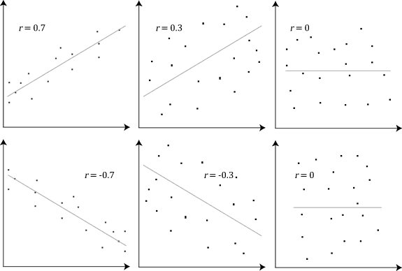
- A correlation coefficient is a statistical measure of the strength of the relationship between the relative movements of two variables. The values range between -1.0 and 1.0. A correlation of -1.0 shows a perfect negative correlation, while a correlation of 1.0 shows a perfect positive correlation. A correlation of 0.0 shows no linear relationship between the movement of the two variables.
Explain Pearson’s Correlation Coefficient
-
Wikipedia Definition: In statistics, the Pearson correlation coefficient also referred to as Pearson’s r or the bivariate correlation is a statistic that measures the linear correlation between two variables X and Y. It has a value between +1 and −1. A value of +1 is a total positive linear correlation, 0 is no linear correlation, and −1 is a total negative linear correlation.
-
Important Inference to keep in mind: The Pearson correlation can evaluate ONLY a linear relationship between two continuous variables (A relationship is linear only when a change in one variable is associated with a proportional change in the other variable)
-
Example use case: We can use the Pearson correlation to evaluate whether an increase in age leads to an increase in blood pressure.
-
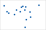
Below is an example (source: Wikipedia) of how the Pearson correlation coefficient (r) varies with the strength and the direction of the relationship between the two variables. Note that when no linear relationship could be established (refer to graphs in the third column), the Pearson coefficient yields a value of zero.
Explain Spearman’s Correlation Coefficient
-
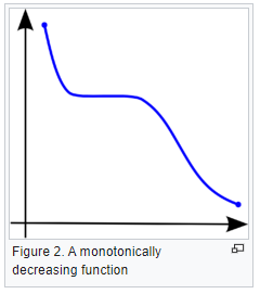
Wikipedia Definition: In statistics, Spearman’s rank correlation coefficient or Spearman’s ρ, named after Charles Spearman is a nonparametric measure of rank correlation (statistical dependence between the rankings of two variables). It assesses how well the relationship between two variables can be described using a monotonic function.
-
Important Inference to keep in mind: The Spearman correlation can evaluate a monotonic relationship between two variables — Continous or Ordinal and it is based on the ranked values for each variable rather than the raw data.
-
What is a monotonic relationship?
- A monotonic relationship is a relationship that does one of the following:
- As the value of one variable increases, so does the value of the other variable, OR,
- As the value of one variable increases, the other variable value decreases.
- But, not exactly at a constant rate whereas in a linear relationship the rate of increase/decrease is constant.
- A monotonic relationship is a relationship that does one of the following:
- Example use case: Whether the order in which employees complete a test exercise is related to the number of months they have been employed or correlation between the IQ of a person with the number of hours spent in front of TV per week.
Compare Pearson and Spearman coefficients
- The fundamental difference between the two correlation coefficients is that the Pearson coefficient works with a linear relationship between the two variables whereas the Spearman Coefficient works with monotonic relationships as well.
- One more difference is that Pearson works with raw data values of the variables whereas Spearman works with rank-ordered variables.
- Now, if we feel that a scatterplot is visually indicating a “might be monotonic, might be linear” relationship, our best bet would be to apply Spearman and not Pearson. No harm would be done by switching to Spearman even if the data turned out to be perfectly linear. But, if it’s not exactly linear and we use Pearson’s coefficient then we’ll miss out on the information that Spearman could capture.
-
Let’s look at some examples (source: A comparison of the Pearson and Spearman correlation methods):
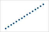
- Pearson = +1, Spearman = +1:
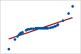
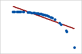
- Pearson = +0.851, Spearman = +1 (This is a monotonically increasing relationship, thus Spearman is exactly 1)
- Pearson = −0.093, Spearman = −0.093
- Pearson = −1, Spearman = −1
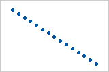
- Pearson = −0.799, Spearman = −1 (This is a monotonically decreasing relationship, thus Spearman is exactly 1)
- Note that both of these coefficients cannot capture any other kind of non-linear relationships. Thus, if a scatterplot indicates a relationship that cannot be expressed by a linear or monotonic function, then both of these coefficients must not be used to determine the strength of the relationship between the variables.
How to choose between Pearson and Spearman correlation?
-
If you want to explore your data it is best to compute both, since the relation between the Spearman (S) and Pearson (P) correlations will give some information. Briefly, \(S\) is computed on ranks and so depicts monotonic relationships while \(P\) is on true values and depicts linear relationships.
-
As an example, if you set:
x=(1:100);
y=exp(x);                         % then,
corr(x,y,'type','Spearman');      % will equal 1, and
corr(x,y,'type','Pearson');       % will be about equal to 0.25
- This is because \(y\) increases monotonically with \(x\) so the Spearman correlation is perfect, but not linearly, so the Pearson correlation is imperfect.
corr(x,log(y),'type','Pearson'); % will equal 1
- Doing both is interesting because if you have \(S > P\), that means that you have a correlation that is monotonic but not linear. Since it is good to have linearity in statistics (it is easier) you can try to apply a transformation on \(y\) (such a log).
Explain the central limit theorem and give examples of when you can use it in a real-world problem?
- The center limit theorem states that if any random variable, regardless of the distribution, is sampled a large enough times, the sample mean will be approximately normally distributed. This allows for studying the properties of any statistical distribution as long as there is a large enough sample size.
Describe the motivation behind random forests and mention two reasons why they are better than individual decision trees?
- The motivation behind random forest or ensemble models in general in layman’s terms, Let’s say we have a question/problem to solve we bring 100 people and ask each of them the question/problem and record their solution. Next, we prepare a solution which is a combination/ a mixture of all the solutions provided by these 100 people. We will find that the aggregated solution will be close to the actual solution. This is known as the “Wisdom of the crowd” and this is the motivation behind Random Forests. We take weak learners (ML models) specifically, Decision Trees in the case of Random Forest & aggregate their results to get good predictions by removing dependency on a particular set of features. In regression, we take the mean and for Classification, we take the majority vote of the classifiers.
- A random forest is generally better than a decision tree, however, you should note that no algorithm is better than the other it will always depend on the use case & the dataset [Check the No Free Lunch Theorem in the first comment]. Reasons why random forests allow for stronger prediction than individual decision trees: 1) Decision trees are prone to overfit whereas random forest generalizes better on unseen data as it is using randomness in feature selection as well as during sampling of the data. Therefore, random forests have lower variance compared to that of the decision tree without substantially increasing the error due to bias. 2) Generally, ensemble models like Random Forest perform better as they are aggregations of various models (Decision Trees in the case of Random Forest), using the concept of the “Wisdom of the crowd.”
Mention three ways to make your model robust to outliers?
-
Investigating the outliers is always the first step in understanding how to treat them. After you understand the nature of why the outliers occurred you can apply one of the several methods mentioned below.
-
Add regularization that will reduce variance, for example, L1 or L2 regularization.
-
Use tree-based models (random forest, gradient boosting ) that are generally less affected by outliers.
-
Winsorize the data. Winsorizing or winsorization is the transformation of statistics by limiting extreme values in the statistical data to reduce the effect of possibly spurious outliers. In numerical data, if the distribution is almost normal using the Z-score we can detect the outliers and treat them by either removing or capping them with some value. If the distribution is skewed using IQR we can detect and treat it by again either removing or capping it with some value. In categorical data check for value_count in the percentage if we have very few records from some category, either we can remove it or can cap it with some categorical value like others.
-
Transform the data, for example, you do a log transformation when the response variable follows an exponential distribution or is right-skewed.
-
Use more robust error metrics such as MAE or Huber loss instead of MSE.
-
Remove the outliers, only do this if you are certain that the outliers are true anomalies that are not worth adding to your model. This should be your last consideration since dropping them means losing information.
Given two arrays, write a python function to return the intersection of the two. For example, X = [1,5,9,0] and Y = [3,0,2,9] it should return [9,0]
- A1 (The most repeated one):
set(X).intersect(set(Y))
- A2:
set(X) & set(Y)
-
Using sets is a very good way to do it since it utilizes a hash map implementation underneath it.
-
A3:
def common_func(X, Y):
Z=[]
for i in X:
for j in Y:
if i==j and i not in Z:
Z.append(i)
return Z
- This is also a simple way to do it, however, it leads to the time complexity of O(N*M) so it is better to use sets.
- Some other answers were mentioned that will work for the mentioned case but will return duplicates for other cases, for example, if X = [1,0,9,9] and Y = [3,0,9,9] it will return [0, 9, 9] not [0,9].
A1:
Res=[i for i in x if i in Y]
A2:
Z = [value for value in X if value in Y]
print(Z)
A3:
d = {}
for value in y:
if value not in d:
d[value] = 1
intersection = []
for value in x:
if value in d:
intersection.append(value)

print(intersection)
- The time complexity for this is O(n + m) and the space complexity is O(m), the problem of it is that it returns duplicates.
Given an array, find all the duplicates in this array for example: input: [1,2,3,1,3,6,5] output: [1,3]
- Approach 1:
set1=set()
res=[]
for i in list:
if i in set1:
res.append(i)
else:
set1.add(i)
print(res)
- Approach 2:
arr1=np.array([1,2,3,1,3,6,5])
nums,index,counts=np.unique(arr1,return_index=True,return_counts=True)
print(nums,index,counts)
nums[counts!=1]
- Approach 3:
a=[1,2,3,1,3,6,5]
j=[i for (i,v) in Counter(a).items() if v>1]
Approach 4: Use map (dict), and get the frequency count of each element. Iterate the map, and print all keys whose values are > 1.
What are the differences and similarities between gradient boosting and random forest? and what are the advantage and disadvantages of each when compared to each other?
- Similarities:
- Both these algorithms are decision-tree based algorithms
- Both these algorithms are ensemble algorithms
- Both are flexible models and do not need much data preprocessing.
- Differences:
- Random forests (Uses Bagging): Trees are arranged in a parallel fashion where the results of all trees are aggregated at the end through averaging or majority vote. Gradient boosting (Uses Boosting): Trees are arranged in a series sequential fashion where every tree tries to minimize the error of the previous tree.
- Radnom forests: Every tree is constructed independently of the other trees. Gradient boosting: Every tree is dependent on the previous tree.
- Advantages of gradient boosting over random forests:
- Gradient boosting can be more accurate than Random forests because we train them to minimize the previous tree’s error.
- Gradient boosting is capable of capturing complex patterns in the data.
- Gradient boosting is better than random forest when used on unbalanced data sets.
- Advantages of random forests over gradient boosting :
- Random forest isless prone to overfit as compared to gradient boosting.
- Random forest has faster training as trees are created parallelly & independent of each other.
- The disadvantage of GB over RF:
- Gradient boosting is more prone to overfitting than random forests due to their focus on mistakes during training iterations and the lack of independence in tree building.
- If the data is noisy the boosted trees might overfit and start modeling the noise.
- In GB training might take longer because every tree is created sequentially.
- Tunning the hyperparameters of gradient boosting is harder than those of random forest.
Small file and big file problem in Big data
- The “small file problem” is kind of notorious in the big data space.
- Did you know there’s also the “Big/large file problem”?
- Say you have a billion records. The small file problem would be like.. 10 records per file and 100 million files. Combining all these files is slow, terrible, and has made many data engineers cry.
- The large file problem would be the opposite problem. 1 billion records in 1 file. This is also a huge problem because how do you parallelize 1 file? You can’t without splitting it up first.
- To avoid crying, the solution is sizing your files the right way. Aiming for between 100-200 MBs for file is usually best. In this contrived example, you’d have a 1000 files each with 1 million records.
- It is worth seeing the spread of files and the size and understanding what optimal file size works out best.
- Too low and you have the risk of more files, too high and the parallelism isn’t going to be effective.
- It is recommended to understand up parallelism, and block size and seeing how the distribution of your data (in files) is before adding an arbitrary default file size value.
What are the Bias and Variance in a Machine Learning Model and explain the bias-variance trade-off?
-
The goal of any supervised machine learning model is to estimate the mapping function (f) that predicts the target variable (y) given input (x). The prediction error can be broken down into three parts:
-
Bias: The bias is the simplifying assumption made by the model to make the target function easy to learn. Low bias suggests fewer assumptions made about the form of the target function. High bias suggests more assumptions made about the form of the target data. The smaller the bias error the better the model is. If the bias error is high, this means that the model is underfitting the training data.
-
Variance: Variance is the amount that the estimate of the target function will change if different training data was used. The target function is estimated from the training data by a machine learning algorithm, so we should expect the algorithm to have some variance. Ideally, it should not change too much from one training dataset to the next, meaning that the algorithm is good at picking out the hidden underlying mapping between the inputs and the output variables. If the variance error is high this indicates that the model overfits the training data.
-
Irreducible error: It is the error introduced from the chosen framing of the problem and may be caused by factors like unknown variables that influence the mapping of the input variables to the output variable. The irreducible error cannot be reduced regardless of what algorithm is used.
-
-
The goal of any supervised machine learning algorithm is to achieve low bias and low variance. In turn, the algorithm should achieve good prediction performance. The parameterization of machine learning algorithms is often a battle to balance out bias and variance.
- For example, if you want to predict the housing prices given a large set of potential predictors. A model with high bias but low variance, such as linear regression will be easy to implement, but it will oversimplify the problem resulting in high bias and low variance. This high bias and low variance would mean in this context that the predicted house prices are frequently off from the market value, but the value of the variance of these predicted prices is low.
- On the other side, a model with low bias and high variance such as a neural network will lead to predicted house prices closer to the market value, but with predictions varying widely based on the input features.
Briefly explain the A/B testing and its application? What are some common pitfalls encountered in A/B testing?
-
A/B testing helps us to determine whether a change in something will cause a change in performance significantly or not. So in other words you aim to statistically estimate the impact of a given change within your digital product (for example). You measure success and counter metrics on at least 1 treatment vs 1 control group (there can be more than 1 XP group for multivariate tests).
- Applications:
-
Consider the example of a general store that sells bread packets but not butter, for a year. If we want to check whether its sale depends on the butter or not, then suppose the store also sells butter and sales for next year are observed. Now we can determine whether selling butter can significantly increase/decrease or doesn’t affect the sale of bread.
-
While developing the landing page of a website you create 2 different versions of the page. You define a criteria for success eg. conversion rate. Then define your hypothesis,
- Null hypothesis (H): No difference between the performance of the 2 versions.
- Alternative hypothesis (H’): version A will perform better than B.
-
-
Note that you will have to split your traffic randomly (to avoid sample bias) into 2 versions. The split doesn’t have to be symmetric, you just need to set the minimum sample size for each version to avoid undersample bias.
-
Now if version A gives better results than version B, we will still have to statistically prove that results derived from our sample represent the entire population. Now one of the very common tests used to do so is 2 sample t-test where we use values of significance level (alpha) and p-value to see which hypothesis is right. If p-value<alpha, H is rejected.
- Common pitfalls:
- Wrong success metrics inadequate to the business problem
- Lack of counter metric, as you might add friction to the product regardless along with the positive impact
- Sample mismatch: heterogeneous control and treatment, unequal variances
- Underpowered test: too small sample or XP running too short 5. Not accounting for network effects (introduce bias within measurement)
Mention three ways to handle missing or corrupted data in adataset?
-
In general, real-world data often has a lot of missing values. The cause of missing values can be data corruption or failure to record data. The handling of missing data is very important during the preprocessing of the dataset as many machine learning algorithms do not support missing values. However, you should start by asking the data owner/stakeholder about the missing or corrupted data. It might be at the data entry level, because of file encoding, etc. which if aligned, can be handled without the need to use advanced techniques.
-
There are different ways to handle missing data, we will discuss only three of them:
-
Deleting the row with missing values
- The first method to handle missing values is to delete the rows or columns that have null values. This is an easy and fast method and leads to a robust model, however, it will lead to the loss of a lot of information depending on the amount of missing data and can only be applied if the missing data represent a small percentage of the whole dataset.
-
Using learning algorithms that support missing values
- Some machine learning algorithms are robust to missing values in the dataset. The K-NN algorithm can ignore a column from a distance measure when there are missing values. Naive Bayes can also support missing values when making a prediction. Another algorithm that can handle a dataset with missing values or null values is the random forest model and Xgboost (check the post in the first comment), as it can work on non-linear and categorical data. The problem with this method is that these models’ implementation in the scikit-learn library does not support handling missing values, so you will have to implement it yourself.
-
Missing value imputation
- Data imputation means the substitution of estimated values for missing or inconsistent data in your dataset. There are different ways to estimate the values that will replace the missing value. The simplest one is to replace the missing value with the most repeated value in the row or the column. Another simple way is to replace it with the mean, median, or mode of the rest of the row or the column. This advantage of this is that it is an easy and fast way to handle the missing data, but it might lead to data leakage and does not factor the covariance between features. A better way is to use a machine learning model to learn the pattern between the data and predict the missing values, this is a very good method to estimate the missing values that will not lead to data leakage and will factor the covariance between the feature, the drawback of this method is the computational complexity especially if your dataset is large.
-
How do you avoid #overfitting? Try one (or more) of the following:
-
Training with more data, which makes the signal stronger and clearer, and can enable the model to detect the signal better. One way to do this is to use #dataaugmentation strategies
-
Reducing the number of features in order to avoid the curse of dimensionality (which occurs when the amount of data is too low to support highly-dimensional models), which is a common cause for overfitting
-
Using cross-validation. This technique works because the model is unlikely to make the same mistake on multiple different samples, and hence, errors will be evened out
-
Using early stopping to end the training process before the model starts learning the noise
-
Using regularization and minimizing the adjusted loss function. Regularization works because it discourages learning a model that’s overly complex or flexible
-
Using ensemble learning, which ensures that the weaknesses of a model are compensated by the other ones
Data science /#MLinterview are hard - regardless which side of the table you are on.
-
As a jobseeker, it can be really hard to shine, especially when the questions asked have little to no relevance to the actual job. How are you supposed to showcase your ability to build models when the entire interview revolves are binary search trees?
-
As a hiring manager, it’s close to impossible to evaluate modeling skills by just talking to someone, and false positives are really frequent. A question that dramatically reduces the noise on both sides:
“What is the most machine learning complex concept you came across, and how would you explain it to yourself that would have made it easier for you to understand it before you learned it?”
-
The answer will tell you a lot more about the candidate than you might think:
- 90% of candidates answer “overfitting”. If they’re junior and explain it really well and they’re junior, it means they’re detailed-oriented and try to gain a thorough understanding of the field, but they sure could show more ambition; if they don’t, it means their understanding of the fundamentals is extremely basic.
- If they answer back-propagation, and they can explain it well, it means they’re more math-oriented than the average and will probably be a good candidate for a research role as an applied DS role.
- If their answer has something to do with a brand-new ML concept, , and they can explain it well, it means they’re growth-oriented and well-read.
- Generally speaking, if they answer something overly complicated and pompous, but can’t explain it well, it means they’re trying to impress but have an overall shallow understanding - a good rule of thumb is not hire them.
- Now, if you are a candidate, or an ML professional, keep asking yourself that question: “What is the most sophisticated concept, model or architecture you know of?” If you keep giving the same answer, maybe you’ve become complacent, and it’s time for you to learn something new.
- How would you explain it to a newbie? As Einstein said, if “you can’t explain it simply, you don’t understand it well enough”.
Order of execution of an SQL Query in Detail
-
Each query begins with finding the data that we need in a database, and then filtering that data down into something that can be processed and understood as quickly as possible.
-
Because each part of the query is executed sequentially, it’s important to understand the order of execution so that you know what results are accessible where.
-
Consider the below mentioned query :
SELECT DISTINCT column, AGG_FUNC(column_or_expression), …
FROM mytable
JOIN another_table
ON mytable.column = another_table.column
WHERE constraint_expression
GROUP BY column
HAVING constraint_expression
ORDER BY column ASC/DESC
LIMIT count OFFSET COUNT;
- Query order of execution:
1.FROMandJOINs
- TheFROMclause, and subsequentJOINs are first executed to determine the total working set of data that is being queried. This includes subqueries in this clause, and can cause temporary tables to be created under the hood containing all the columns and rows of the tables being joined.
2.WHERE
- Once we have the total working set of data, the first-passWHEREconstraints are applied to the individual rows, and rows that do not satisfy the constraint are discarded. Each of the constraints can only access columns directly from the tables requested in theFROMclause. Aliases in theSELECTpart of the query are not accessible in most databases since they may include expressions dependent on parts of the query that have not yet executed.
3.GROUP BY
- The remaining rows after theWHEREconstraints are applied are then grouped based on common values in the column specified in theGROUP BYclause. As a result of the grouping, there will only be as many rows as there are unique values in that column. Implicitly, this means that you should only need to use this when you have aggregate functions in your query.
4.HAVING
- If the query has aGROUP BYclause, then the constraints in theHAVINGclause are then applied to the grouped rows, discard the grouped rows that don’t satisfy the constraint. Like theWHEREclause, aliases are also not accessible from this step in most databases.
5.SELECT
- Any expressions in theSELECTpart of the query are finally computed.
6.DISTINCT
- Of the remaining rows, rows with duplicate values in the column marked asDISTINCTwill be discarded.
7.ORDER BY
- If an order is specified by theORDER BYclause, the rows are then sorted by the specified data in either ascending or descending order. Since all the expressions in theSELECTpart of the query have been computed, you can reference aliases in this clause.
8.LIMIT/OFFSET
- Finally, the rows that fall outside the range specified by theLIMITandOFFSETare discarded, leaving the final set of rows to be returned from the query.
Explain briefly the logistic regression model and state an example of when you have used it recently?
- Logistic regression is used to calculate the probability of occurrence of an event in the form of a dependent output variable based on independent input variables. Logistic regression is commonly used to estimate the probability that an instance belongs to a particular class. If the probability is bigger than 0.5 then it will belong to that class (positive) and if it is below 0.5 it will belong to the other class. This will make it a binary classifier.
- It is important to remember that the Logistic regression isn’t a classification model, it’s an ordinary type of regression algorithm, and it was developed and used before machine learning, but it can be used in classification when we put a threshold to determine specific categories.
- There is a lot of classification applications to it: classify email as spam or not, identify whether the patient is healthy or not, etc.
Describe briefly the hypothesis testing and p-value in layman’s terms? And give a practical application for them?
- In Layman’s terms:
- Hypothesis test is where you have a current state (null hypothesis) and an alternative state (alternative hypothesis). You assess the results of both of the states and see some differences. You want to decide whether the difference is due to the alternative approach or not.
- You use the p-value to decide this, where the p-value is the likelihood of getting the same results the alternative approach achieved if you keep using the existing approach. It’s the probability to find the result in the gaussian distribution of the results you may get from the existing approach.
- The rule of thumb is to reject the null hypothesis if the p-value < 0.05, which means that the probability to get these results from the existing approach is <95%. But this % changes according to task and domain.
- To explain the hypothesis testing in layman’s term with an example, suppose we have two drugs A and B, and we want to determine whether these two drugs are the same or different. This idea of trying to determine whether the drugs are the same or different is called hypothesis testing. The null hypothesis is that the drugs are the same, and the p-value helps us decide whether we should reject the null hypothesis or not.
- p-values are numbers between 0 and 1, and in this particular case, it helps us to quantify how confident we should be to conclude that drug A is different from drug B. The closer the p-value is to 0, the more confident we are that the drugs A and B are different.
What is an activation function and discuss the use of an activation function? Explain three different types of activation functions?
- In mathematical terms, the activation function serves as a gate between the current neuron input and its output, going to the next level. Basically, it decides whether neurons should be activated or not. It is used to introduce non-linearity into a model.
- Activation functions are added to introduce non-linearity to the network, it doesn’t matter how many layers or how many neurons your net has, the output will be linear combinations of the input in the absence of activation functions. In other words, activation functions are what make a linear regression model different from a neural network. We need non-linearity, to capture more complex features and model more complex variations that simple linear models can not capture.
- There are a lot of activation functions:
- Sigmoid function: \(f(x) = 1/(1+exp(-x))\).
- The output value of it is between 0 and 1, we can use it for classification. It has some problems like the gradient vanishing on the extremes, also it is computationally expensive since it uses exp.
- ReLU: \(f(x) = max(0,x)\).
- it returns 0 if the input is negative and the value of the input if the input is positive. It solves the problem of vanishing gradient for the positive side, however, the problem is still on the negative side. It is fast because we use a linear function in it.
- Leaky ReLU:
- Sigmoid function: \(f(x) = 1/(1+exp(-x))\).
- It solves the problem of vanishing gradient on both sides by returning a value “a” on the negative side and it does the same thing as ReLU for the positive side.
- Softmax: it is usually used at the last layer for a classification problem because it returns a set of probabilities, where the sum of them is 1. Moreover, it is compatible with cross-entropy loss, which is usually the loss function for classification problems.
If you roll a dice three times, what is the probability to get two consecutive threes?
- The answer is 11/216.
- There are different ways to answer this question:
- If we roll a dice three times we can get two consecutive 3’s in three ways:
- The first two rolls are 3s and the third is any other number with a probability of 1/6 * 1/6 * 5/6.
- The first one is not three while the other two rolls are 3s with a probability of 5/6 * 1/6 * 1/6.
- The last one is that the three rolls are 3s with probability 1/6 ^ 3.
- So the final result is \(2 * (5/6 * (1/6)^2) + (1/6)*3 = 11/216\).
- By Inclusion-Exclusion Principle:
- Probability of at least two consecutive threes: = Probability of two consecutive threes in first two rolls + Probability of two consecutive threes in last two rolls - Probability of three consecutive threes = 2Probability of two consecutive threes in first two rolls - Probability of three consecutive threes = 21/61/6 - 1/61/6*1/6 = 11/216
- It can be seen also like this:
- The sample space is made of (x, y, z) tuples where each letter can take a value from 1 to 6, therefore the sample space has 6x6x6=216 values, and the number of outcomes that are considered two consecutive threes is (3,3, X) or (X, 3, 3), the number of possible outcomes is therefore 6 for the first scenario (3,3,1) till (3,3,6) and 6 for the other scenario (1,3,3) till (6,3,3) and subtract the duplicate (3,3,3) which appears in both, and this leaves us with a probability of 11/216.
- If we roll a dice three times we can get two consecutive 3’s in three ways:
You and your friend are playing a game with a fair coin. The two of you will continue to toss the coin until the sequence HH or TH shows up. If HH shows up first, you win, and if TH shows up first your friend win. What is the probability of you winning the game?
- If T is ever flipped, you cannot then reach HH before your friend reaches TH. Therefore, the probability of you winning this is to flip HH initially. Therefore the sample space will be {HH, HT, TH, TT} and the probability of you winning will be (1/4) and your friend (3/4).
Dimensionality reduction techniques
-
Dimensionality reduction techniques help deal with the curse of dimensionality. Some of these are supervised learning approaches whereas others are unsupervised. Here is a quick summary:
- PCA - Principal Component Analysis is an unsupervised learning approach and can Handle skewed data easily for dimensionality reduction.
- LDA - Linear Discriminant Analysis is also a dimensionality reduction technique based on eigenvectors but it also maximizes class separation while doing so. Moreover, it is a supervised Learning approach and it performs better with uniformly distributed data.
- ICA - Independent Component Analysis aims to maximize the statistical independence between variables and is a Supervised learning approach.
- MDS - Multi dimensional scaling aims to preserve the Euclidean pairwise distances. It is an Unsupervised learning approach.
- ISOMAP - Also known as Isometric Mapping is another dimensionality reduction technique which preserves geodesic pairwise distances. It is an unsupervised learning approach. It can handle noisy data well.
- t-SNE - Called the t-distributed stochastic neighbor embedding preserves local structure and is an Unsupervised learning approach.
Active learning
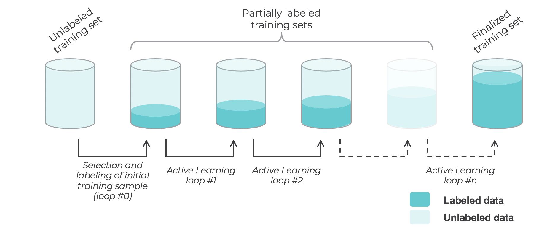
- Active learning is a semi-supervised ML training paradigm which, like all semi-supervised learning techniques, relies on the usage of partially labeled data.
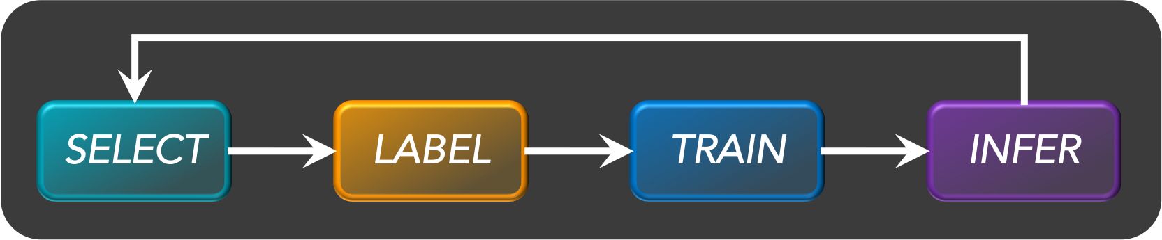
- Active Learning consists of dynamically selecting the most relevant data by sequentially:
- selecting a sample of the raw (unannotated) dataset (the algorithm used for that selection step is called a querying strategy).
- getting the selected data annotated.
- training the model with that sample of annotated training data.
- running inference on the remaining (unannotated) data.
- That last step is used to evaluate which records should be then selected for the next iteration (called a loop). However, since there is no ground truth for the data used in the inference step, one cannot simply decide to feed the – data where the model failed to make the correct prediction, and has instead to use metadata (such as the confidence level of the prediction) to make that decision.
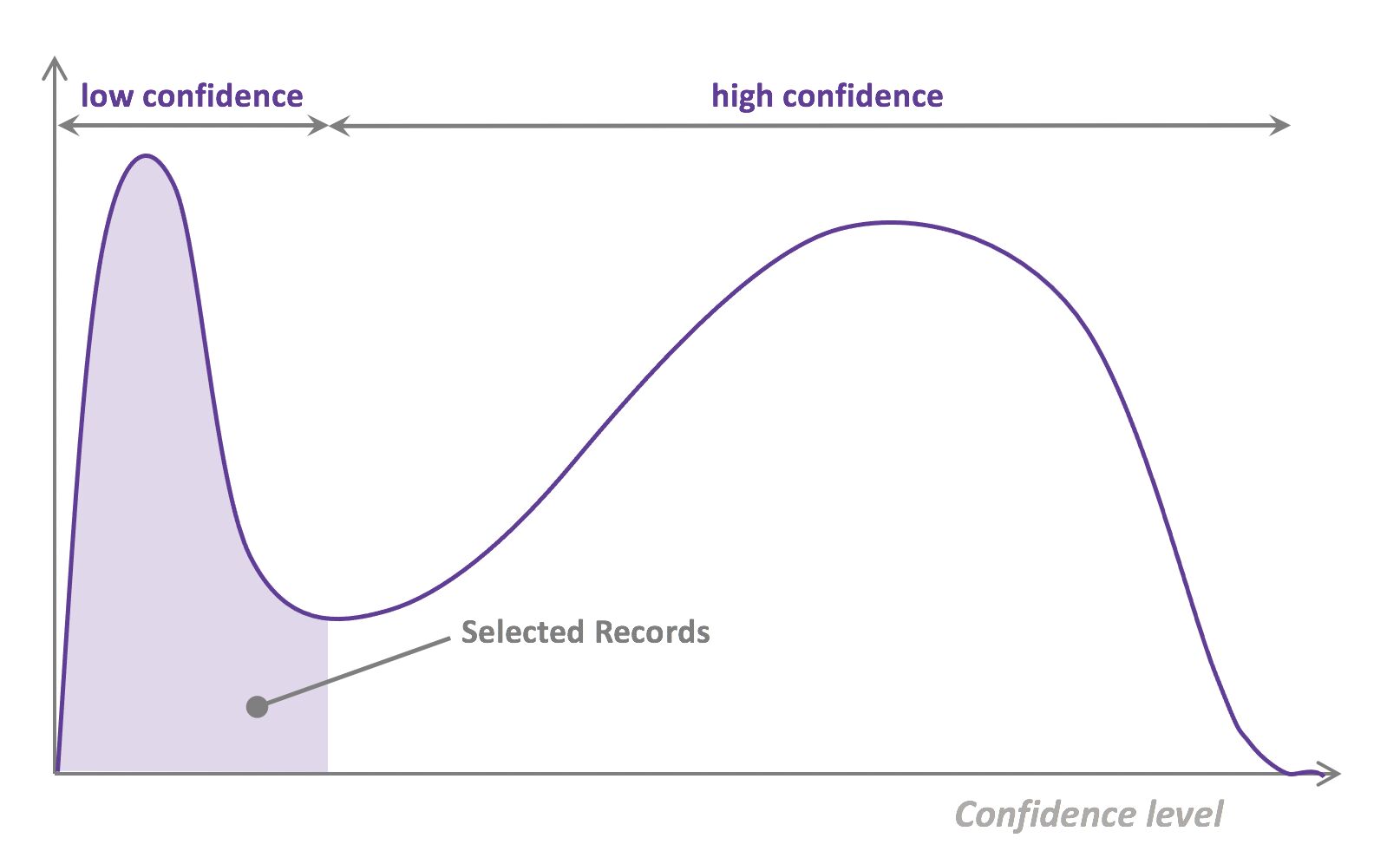
- The easiest and most common querying strategy used for selecting the next batch of useful data consists of picking the records with the lowest confidence level; this is called the least-confidence querying strategy, which is one of many possible querying strategies.
What is the independence assumption for a Naive Bayes classifier?
- Naive bayes assumes that the feature probabilities are independent given the class \(c\), i.e., the features do not depend on each other are totally uncorrelated.
- This is why the Naive Bayes algorithm is called “naive”.
-
Mathematically, the features are independent given class:
\[\begin{aligned} P\left(X_{1}, X_{2} \mid Y\right) &=P\left(X_{1} \mid X_{2}, Y\right) P\left(X_{2} \mid Y\right) \\ &=P\left(X_{1} \mid Y\right) P\left(X_{2} \mid Y\right) \end{aligned}\]- More generally: \(P\left(X_{1} \ldots X_{n} \mid Y\right)=\prod_{i} P\left(X_{i} \mid Y\right)\)
Explain briefly batch gradient descent, stochastic gradient descent, and mini-batch gradient descent? List the pros and cons of each.
- Gradient descent is a generic optimization algorithm capable for finding optimal solutions to a wide range of problems. The general idea of gradient descent is to tweak parameters iteratively in order to minimize a cost function.
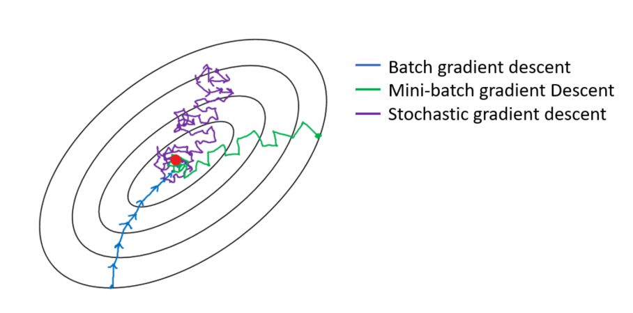
- Batch Gradient Descent:
- In Batch Gradient descent the whole training data is used to minimize the loss function by taking a step towards the nearest minimum by calculating the gradient (the direction of descent).
- Pros:
- Since the whole data set is used to calculate the gradient it will be stable and reach the minimum of the cost function without bouncing around the loss function landscape (if the learning rate is chosen correctly).
- Cons:
- Since batch gradient descent uses all the training set to compute the gradient at every step, it will be very slow especially if the size of the training data is large.
- Stochastic Gradient Descent:
- Stochastic Gradient Descent picks up a random instance in the training data set at every step and computes the gradient-based only on that single instance.
- Pros:
- It makes the training much faster as it only works on one instance at a time.
- It become easier to train using large datasets.
- Cons:
- Due to the stochastic (random) nature of this algorithm, this algorithm is much less stable than the batch gradient descent. Instead of gently decreasing until it reaches the minimum, the cost function will bounce up and down, decreasing only on average. Over time it will end up very close to the minimum, but once it gets there it will continue to bounce around, not settling down there. So once the algorithm stops, the final parameters would likely be good but not optimal. For this reason, it is important to use a training schedule to overcome this randomness.
- Mini-batch Gradient:
- At each step instead of computing the gradients on the whole data set as in the Batch Gradient Descent or using one random instance as in the Stochastic Gradient Descent, this algorithm computes the gradients on small random sets of instances called mini-batches.
- Pros:
- The algorithm’s progress space is less erratic than with Stochastic Gradient Descent, especially with large mini-batches.
- You can get a performance boost from hardware optimization of matrix operations, especially when using GPUs.
- Cons:
- It might be difficult to escape from local minima.
- Batch Gradient Descent:
Explain what is information gain and entropy in the context of decision trees?
- Entropy and Information Gain are two key metrics used in determining the relevance of decision making when constructing a decision tree model and to determine the nodes and the best way to split.
- The idea of a decision tree is to divide the data set into smaller data sets based on the descriptive features until we reach a small enough set that contains data points that fall under one label.
- Entropy is the measure of impurity, disorder, or uncertainty in a bunch of examples. Entropy controls how a Decision Tree decides to split the data. Information gain calculates the reduction in entropy or surprise from transforming a dataset in some way. It is commonly used in the construction of decision trees from a training dataset, by evaluating the information gain for each variable, and selecting the variable that maximizes the information gain, which in turn minimizes the entropy and best splits the dataset into groups for effective classification.
What are some applications of RL beyond gaming and self-driving cars?
- Reinforcement learning is NOT just used in gaming and self-driving cars, here are three common use cases you should know in 2022:
-
Multi-arm bandit testing (MAB)
- A little bit about reinforcement learning (RL): you train an agent to interact with the environment and figure out the optimum policy which maximizes the reward (a metric you select).
- MAB is a classic reinforcement learning problem that can be used to help you find a best options out of a lot of treatments in experimentation.
- Unlike A/B tests, MAB tries to maximizes a metric (reward) during the course of the test. It usually has a lot of treatments to select from. The trade-off is that you can draw causal inference through traditional A/B testing, but it’s hard to analyze each treatment through MAB; however, because it’s dynamic, it might be faster to select the best treatment than A/B testing.
-
Recommendation engines
- While traditional matrix factorization works well for recommendation engines, using reinforcement learning can help you maximize metrics like customer engagement and metrics that measure downstream impact.
- For example, social media can use RL to maximize ‘time spent’ or ‘review score’ when recommending content; so this way, instead of just recommending similar content, you might also help customers discover new content or other popular content they like.
-
Portfolio Management
- RL has been used in finance recently as well. Data scientist can train the agent to interact with a trading environment to maximize the return of the portfolio. For example, if the agent selects an allocation of 70% stock, 10% Cash, and 20% bond, the agent gets a positive or negative reward for this allocation. Through iteration, the agent finds out the best allocation.
- Robo-advisers can also use RL to learn investors risk tolerance.
- Of course, self-driving cars, gaming, robotics use RL heavily, but I’ve seen data scientists from industries mentioned above (retail, social media, finance) start to use more RL in their day-to-day work.
You are using a deep neural network for a prediction task. After training your model, you notice that it is strongly overfitting the training set and that the performance on the test isn’t good. What can you do to reduce overfitting?
- To reduce overfitting in a deep neural network changes can be made in three places/stages: The input data to the network, the network architecture, and the training process:
- The input data to the network:
- Check if all the features are available and reliable
- Check if the training sample distribution is the same as the validation and test set distribution. Because if there is a difference in validation set distribution then it is hard for the model to predict as these complex patterns are unknown to the model.
- Check for train / valid data contamination (or leakage)
- The dataset size is enough, if not try data augmentation to increase the data size
- The dataset is balanced
- Network architecture:
- Overfitting could be due to model complexity. Question each component:
- can fully connect layers be replaced with convolutional + pooling layers?
- what is the justification for the number of layers and number of neurons chosen? Given how hard it is to tune these, can a pre-trained model be used?
- Add regularization - ridge (l1), lasso (l2), elastic net (both)
- Add dropouts
- Add batch normalization
- The training process:
- Improvements in validation losses should decide when to stop training. Use callbacks for early stopping when there are no significant changes in the validation loss and restore_best_weights.
Explain the linear regression model and discuss its assumption?
- Linear regression is a supervised statistical model to predict dependent variable quantity based on independent variables.
- Linear regression is a parametric model and the objective of linear regression is that it has to learn coefficients using the training data and predict the target value given only independent values.
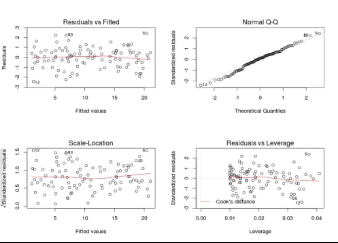
- Some of the linear regression assumptions and how to validate them:
- Linear relationship between independent and dependent variables
- Independent residuals and the constant residuals at every \(x\): We can check for 1 and 2 by plotting the residuals(error terms) against the fitted values (upper left graph). Generally, we should look for a lack of patterns and a consistent variance across the horizontal line.
- Normally distributed residuals: We can check for this using a couple of methods: -Q-Q-plot(upper right graph): If data is normally distributed, points should roughly align with the 45-degree line. -Boxplot: it also helps visualize outliers -Shapiro–Wilk test: If the p-value is lower than the chosen threshold, then the null hypothesis (Data is normally distributed) is rejected.
- Low multicollinearity
- You can calculate the VIF (Variable Inflation Factors) using your favorite statistical tool. If the value for each covariate is lower than 10 (some say 5), you’re good to go.
- The figure below summarizes these assumptions.
Explain briefly the K-Means clustering and how can we find the best value of K?
- K-Means is a well-known clustering algorithm. K-Means clustering is often used because it is easy to interpret and implement. It starts by partitioning a set of data into \(K\) distinct clusters and then arbitrary selects centroids of each of these clusters. It iteratively updates partitions by first assigning the points to the closet cluster and then updating the centroid and then repeating this process until convergence. The process essentially minimizes the total inter-cluster variation across all clusters.
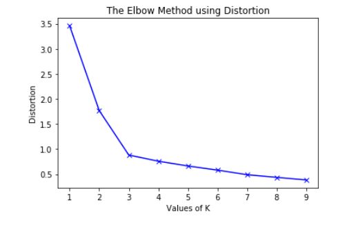
- The elbow method is a well-known method to find the best value of \(K\) in K-means clustering. The intuition behind this technique is that the first few clusters will explain a lot of the variation in the data, but past a certain point, the amount of information added is diminishing. Looking at the graph below of the explained variation (on the y-axis) versus the number of cluster \(K\) (on the x-axis), there should be a sharp change in the y-axis at some level of \(K\). For example in the graph below the drop-off is at \(k=3\).
- The explained variation is quantified by the within-cluster sum of squared errors. To calculate this error notice, we look for each cluster at the total sum of squared errors using Euclidean distance.
- Another popular alternative method to find the value of \(K\) is to apply the silhouette method, which aims to measure how similar points are in its cluster compared to other clusters. It can be calculated with this equation: \((x-y)/max(x,y)\), where \(x\) is the mean distance to the examples of the nearest cluster, and \(y\) is the mean distance to other examples in the same cluster. The coefficient varies between -1 and 1 for any given point. A value of 1 implies that the point is in the right cluster and the value of -1 implies that it is in the wrong cluster. By plotting the silhouette coefficient on the y-axis versus each \(K\) we can get an idea of the optimal number of clusters. However, it is worthy to note that this method is more computationally expensive than the previous one.
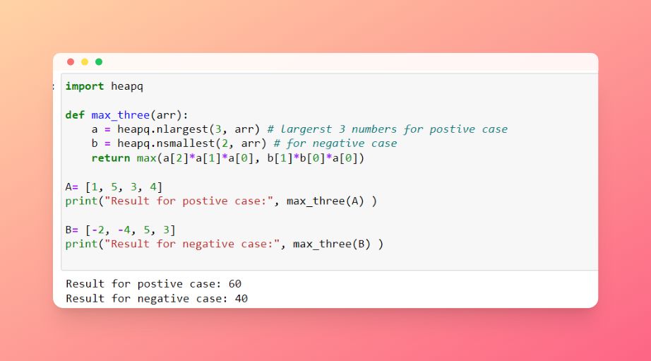
Given an integer array, return the maximum product of any three numbers in the array.
- For example:
A = [1, 5, 3, 4] it should return 60
B = [-2, -4, 5, 3] it should return 40
- If all the numbers are positive, then the solution will be finding the max 3 numbers, if they have negative numbers then it will be the result of multiplying the smallest two negative numbers with the maximum positive number.
- We can use the
heapqlibrary to sort and find the maximum numbers in one step. As shown in the image below.
What are joins in SQL and discuss its types?
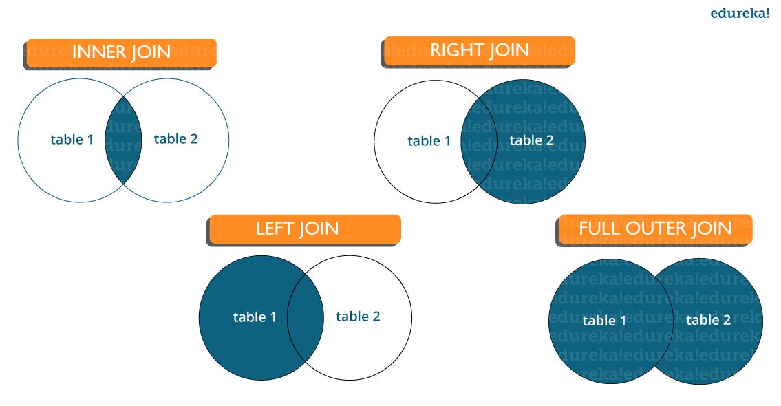
- A JOIN clause is used to combine rows from two or more tables, based on a related column between them. It is used to merge two tables or retrieve data from there. There are 4 types of joins: inner join left join, right join, and full join.
- Inner join: Inner Join in SQL is the most common type of join. It is used to return all the rows from multiple tables where the join condition is satisfied.
- Left Join: Left Join in SQL is used to return all the rows from the left table but only the matching rows from the right table where the join condition is fulfilled.
- Right Join: Right Join in SQL is used to return all the rows from the right table but only the matching rows from the left table where the join condition is fulfilled.
- Full Join: Full join returns all the records when there is a match in any of the tables. Therefore, it returns all the rows from the left-hand side table and all the rows from the right-hand side table.
Why should we use Batch Normalization?
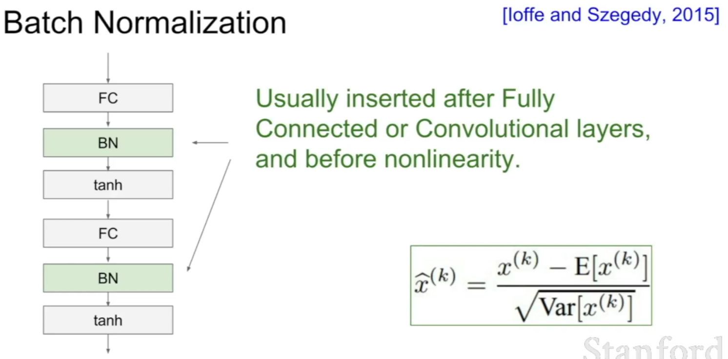
- Batch normalization is a technique for training very deep neural networks that standardizes the inputs to a layer for each mini-batch.
- Usually, a dataset is fed into the network in the form of batches where the distribution of the data differs for every batch size. By doing this, there might be chances of vanishing gradient or exploding gradient when it tries to backpropagate. In order to combat these issues, we can use BN (with irreducible error) layer mostly on the inputs to the layer before the activation function in the previous layer and after fully connected layers.
- Batch Normalisation has the following effects on the Neural Network:
- Robust Training of the deeper layers of the network.
- Better covariate-shift proof NN Architecture.
- Has a slight regularization effect.
- Centered and controlled values of Activation.
- Tries to prevent exploding/vanishing gradient.
- Faster training/convergence.
What is weak supervision?
- Weak Supervision (which most people know as the Snorkel algorithm) is an approach designed to help annotate data at scale, and it’s a pretty clever one too.
- Imagine that you have to build a content moderation system that can flag LinkedIn posts that are offensive. Before you can build a model, you’ll first have to get some data. So you’ll scrape posts. A lot of them, because content moderation is particularly data-greedy. Say, you collect 10M of them. That’s when trouble begins: you need to annotate each and every one of them - and you know that’s gonna cost you a lot of time and a lot of money!
- So you want to use autolabeling (basically, you want to apply a pre-trained model) to generate ground truth. The problem is that such a model doesn’t just lie around, as this isn’t your vanilla object detection for autonomous driving use case, and you can’t just use YOLO v5.
- Rather than seek the budget to annotate all that data, you reach out to subject matter experts you know on LinkedIn, and you ask them to give you a list of rules of what constitutes, according to each one of them, an offensive post.
Person 1's rules:
- The post is in all caps
- There is a mention of Politics

Person 2's rules:
- The post is in all caps
- It uses slang
- The topic is not professional

...

Person 20's rules:
- The post is about religion
- The post mentions death
- You then combine all rules into a mega processing engine that functions as a voting system: if a comment is flagged as offensive by at least X% of those 20 rule sets, then you label it as offensive. You apply the same logic to all 10M records and are able to annotate then in minutes, at almost no costs.
- You just used a weakly supervised algorithm to annotate your data.
- You can of course replace people’s inputs by embeddings, or some other automatically generated information, which comes handy in cases when no clear rules can be defined (for example, try coming up with rules to flag a cat in a picture).
What is active learning?
- When you don’t have enough labeled data and it’s expensive and/or time consuming to label new data, active learning is the solution. Active learning is a semi-supervised ML training paradigm which, like all semi-supervised learning techniques, relies on the usage of partially labeled data. Active Learning helps to select unlabeled samples to label that will be most beneficial for the model, when retrained with the new sample.
- Active Learning consists of dynamically selecting the most relevant data by sequentially:
- selecting a sample of the raw (unannotated) dataset (the algorithm used for that selection step is called a querying strategy)
- getting the selected data annotated
- training the model with that sample of annotated training data
- running inference on the remaining (unannotated) data.
- That last step is used to evaluate which records should be then selected for the next iteration (called a loop). However, since there is no ground truth for the data used in the inference step, one cannot simply decide to feed the data where the model failed to make the correct prediction, and has instead to use metadata (such as the confidence level of the prediction) to make that decision.
- The easiest and most common querying strategy used for selecting the next batch of useful data consists of picking the records with the lowest confidence level; this is called the least-confidence querying strategy, which is one of many possible querying strategies. (Technically, those querying strategies are usually brute-force, arbitrary algorithms which can be replaced by actual ML models trained on metadata generated during the training and inference phases for more sophistication).
- Thus, the most important criterion is selecting samples with maximum prediction uncertainty. You can use the model’s prediction confidence to ascertain uncertain samples. Entropy is another way to measure such uncertainty. Another criterion could be diversity of the new sample with respect to exiting training data. You could also select samples close to labeled samples in the training data with poor performance. Another option could be selecting samples from regions of the feature space where better performance is desired. You could combine all the strategies in your active learning decision making process.
- The training is an iterative process. With active learning you select new sample to label, label it and retrain the model. Adding one labeled sample at a time and retraining the model could be expensive. There are techniques to select a batch of samples to label. For deep learning the most popular active learning technique is entropy with is Monte Carlo dropout for prediction probability.
- The process of deciding the samples to label could also be implemented with Multi Arm Bandit. The reward function could be defined in terms of prediction uncertainty, diversity, etc.
- Let’s go deeper and explain why the vanilla form of Active Learning, “uncertainty-based”/”least-confidence” Active Learning, actually perform poorly via real-life datasets:
- Let’s take the example of a binary classification model identifying toxic content in tweets, and let’s say we have 100,000 tweets as our dataset.
- Here is how uncertainty-based AL would work:
- We pick 1,000 (or another number, depending on how we tune the process) records - at that stage, randomly.
- We annotate that data as toxic / not-toxic.
- We train our model with it and get a (not-so-good) model.
- We use the model to infer the remaining 99,000 (unlabeled) records.
- We don’t have ground truth for those 99,000, so we can’t select which records are incorrectly predicted, but we can use metadata, such as the confidence level, as a proxy to detect bad predictions. With least confidence Active Learning, we would pick the 1,000 records predicted with the lowest confidence level as our next batch.
- Go to (2) and repeat the same steps, until we’re happy with the model.
- What we did here, is assume that confidence was a good proxy for usefulness, because it is assumed that low confidence records are the hardest for the model to learn, and hence that the model needs to see them to learn more efficiently.
- Let’s consider a scenario where it is not. Assume now that this training data is not clean, and 5% of the data is actually in Spanish. If the model (and the majority of the data) was meant to be for English, then chances are, the Spanish tweets will be inferred with a low confidence: you will actually pollute the dataset with data that doesn’t belong there. In other words, low confidence can happen for a variety of different reasons. That’s what happens when you do active learning with messy data.
- To resolve this, one solution is to stop using confidence level alone: confidence levels are just one meta-feature to evaluate usefulness.
- In a nutshell, active learning is an incremental semi-supervised learning paradigm where training data is selected incrementally and the model is sequentially retrained (loop after loop), until either the model reaches a specific performance or labeling budget is exhausted.
What are the types of active learning?
- There are many different “flavors” of active learning, but did you know that active learning could be broken down into two main categories, “streaming active learning”, and “pooling (batch) active learning”?
- Pooling Active Learning, is when all records available for training data have to be evaluated before a decision can be made about the ones to keep. For example, if your querying strategy is least-confidence, you goal is to select the N records that were predicted with the lowest confidence level in the previous loop, which means all records have to be ranked accordingly to their confidence level. Pooling Active Learning hence requires more compute resources for inference (the entire remainder of the dataset, at each loop, needs to be inferred), but provides a better control of loop sizes and the process as a whole.
- Streaming Active Learning, is when a decision is made “on the fly”, record by record. If your selection strategy was to select all records predicted with a confidence level lower than X% for the previous loop, you’d be doing Streaming AL. This technique obviously requires less compute, and can be used in combination with Online Learning, but it comes with a huge risk: there is no guarantee regarding the amount of data that will be selected. Set the threshold too low, and you won’t select any data for the next loop. Set the threshold too high, and all the remaining data gets selected, and you lose the benefit of AL.
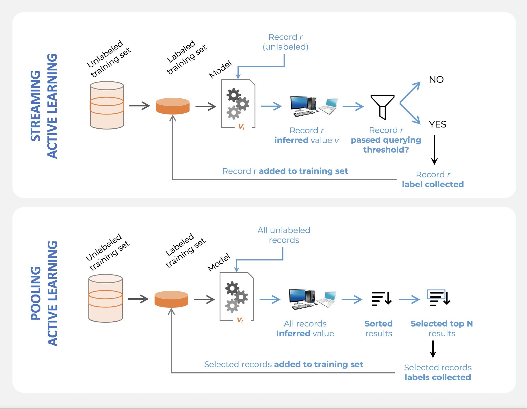
What is the difference between online learning and active learning?
- Online learning is essentially the concept of training a machine learning model on streaming data. In that case, data arrives little-by-little, sequentially, and the model is updated as opposed to be trained entirely from scratch.
- Active learning also consists in training a model sequentially, but the difference is that the training dataset is already fully available. Active learning simply selects small samples of data incrementally; the model is either retrained with the totality of selected records at a given point in time, or updated with the newly selected data.
- Online learning is required when models are to be trained at the point of collection (e.g, on the edge of a device), but active learning, just like supervised learning, usually involves the model being trained offline.
Why is active learning not frequently used with deep learning?
-
Active Learning was relatively popular among ML scientists during the pre-Deep Learning era, and somehow fell out of favor afterwards.
-
The reason why is actually relatively simple: Active Learning usually doesn’t work as well with Deep Learning Models (at least the most common querying strategies don’t). So people gave up on Deep Active Learning pretty quickly. The two most important reasons are the following:
-
The least-confidence, by far the most popular querying strategy, requires the computation of a confidence score. However, the softmax technique which most ML scientists rely on, is relatively unreliable (see this article for details to learn about a better way to compute confidence: https://arxiv.org/pdf/1706.04599.pdf)
-
Active learning, as a process, is actually meant to “grow” a better dataset dynamically. At each loop, more records are selected, which means the same model is retrained with incrementally larger data. However, many hyperparameters in neural nets are very sensitive to the amount of data used. For example, a certain number of epochs might lead to overfitting with early loops and underfitting later on. The proper way of doing Deep Active Learning would be to do hyperparameter tuning dynamically, which is rarely done.
What does active learning have to do with explore-exploit?
- Using the “uncertainty-based”/”least/lowest-confidence” querying strategy as a selection criteria in an active learning process could cause issues when working with a real-life (messy) dataset, as indicated above.
- Uncertainty-based active learning aims at selecting records based on how “certain” (or confident) the model already is about what it knows. Assuming the model can be trusted to self-evaluate properly, then:
- Selecting low confidence records is about picking what the model seems not to know yet; it is a pure exploration process.
- Selecting high confidence records is about picking what the model seems to already know, and that would be about reinforcing that knowledge; it is a pure exploitation process.
- While the “uncertainty-based”/”least/lowest-confidence” querying strategy strategy is the most common using active learning, it might be better to balance exploration and exploitation, and that active learning can and should, in fact, be formulated as a reinforcement learning problem.
What are the differences between a model that minimizes squared error and the one that minimizes the absolute error? and in which cases each error metric would be more appropriate?
- Both mean square error (MSE) and mean absolute error (MAE) measures the distances between vectors and express average model prediction in units of the target variable. Both can range from 0 to infinity, the lower they are the better the model.
- The main difference between them is that in MSE the errors are squared before being averaged while in MAE they are not. This means that a large weight will be given to large errors. MSE is useful when large errors in the model are trying to be avoided. This means that outliers affect MSE more than MAE (because large errors have a greater influence than small errors), that is why MAE is more robust to outliers.
- Computation-wise MSE is easier to use as the gradient calculation will be more straightforward than MAE, since MAE requires linear programming to calculate it.
Define tuples and lists in Python What are the major differences between them?
- Lists:
- In Python, a list is created by placing elements inside square brackets
[], separated by commas. A list can have any number of items and they may be of different types (integer, float, string, etc.). A list can also have another list as an item. This is called a nested list.- Lists are mutable (we can change, add, delete and modify stuff).
- Lists are better for performing operations, such as insertion and deletion.
- Lists consume more memory.
- Lists have several built-in methods.
- In Python, a list is created by placing elements inside square brackets
- Tuples:
- A tuple is a collection of objects which ordered and immutable. Tuples are sequences, just like lists. The differences between tuples and lists are, the tuples cannot be changed unlike lists and tuples use parentheses, whereas lists use square brackets.
- Tuples are immutable (we cannot change, add, delete and modify stuff).
- Tuple data type is appropriate for accessing the elements.
- Tuples consume less memory as compared to the list.
- Tuple does not have many built-in methods.
- A tuple is a collection of objects which ordered and immutable. Tuples are sequences, just like lists. The differences between tuples and lists are, the tuples cannot be changed unlike lists and tuples use parentheses, whereas lists use square brackets.
Given a left-skewed distribution that has a median of 60, what conclusions can we draw about the mean and the mode of the data?
- Left skewed distribution means the tail of the distribution is to the left and the tip is to the right. So the mean which tends to be near outliers (very large or small values) will be shifted towards the left or in other words, towards the tail.
- While the mode (which represents the most repeated value) will be near the tip and the median is the middle element independent of the distribution skewness, therefore it will be smaller than the mode and more than the mean.
- Thus,
- Mean < 60
- Mode > 60
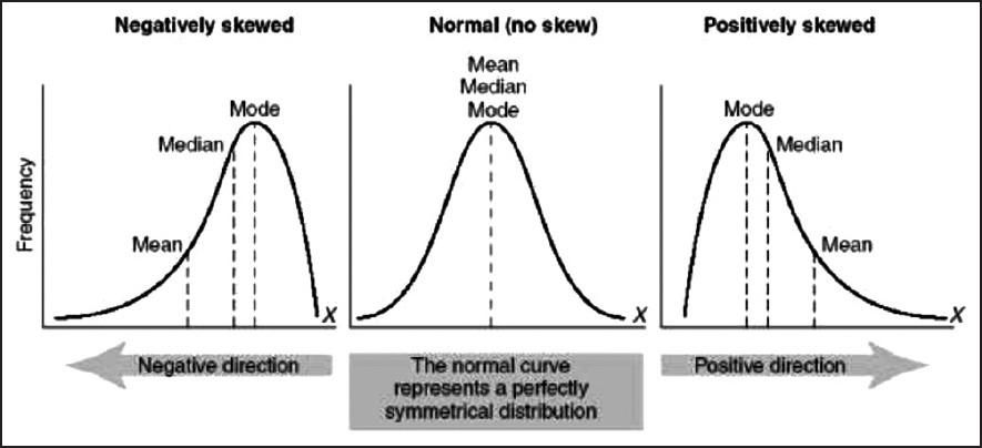
Explain the kernel trick in SVM and why we use it and how to choose what kernel to use?
- Kernels are used in SVM to map the original input data into a particular higher dimensional space where it will be easier to find patterns in the data and train the model with better performance.
- For e.g.: If we have binary class data which form a ring-like pattern (inner and outer rings representing two different class instances) when plotted in 2D space, a linear SVM kernel will not be able to differentiate the two classes well when compared to a RBF (radial basis function) kernel, mapping the data into a particular higher dimensional space where the two classes are clearly separable.
- Typically without the kernel trick, in order to calculate support vectors and support vector classifiers, we need first to transform data points one by one to the higher dimensional space, and do the calculations based on SVM equations in the higher dimensional space, then return the results. The ‘trick’ in the kernel trick is that we design the kernels based on some conditions as mathematical functions that are equivalent to a dot product in the higher dimensional space without even having to transform data points to the higher dimensional space. i.e we can calculate support vectors and support vector classifiers in the same space where the data is provided which saves a lot of time and calculations.
- Having domain knowledge can be very helpful in choosing the optimal kernel for your problem, however in the absence of such knowledge following this default rule can be helpful: For linear problems, we can try linear or logistic kernels and for nonlinear problems, we can use RBF or Gaussian kernels.
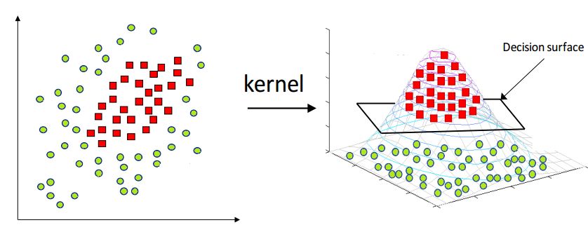
Can you explain the parameter sharing concept in deep learning?
- Parameter sharing is the method of sharing weights by all neurons in a particular feature map. Therefore helps to reduce the number of parameters in the whole system, making it computationally cheap. It basically means that the same parameters will be used to represent different transformations in the system. This basically means the same matrix elements may be updated multiple times during backpropagation from varied gradients. The same set of elements will facilitate transformations at more than one layer instead of those from a single layer as conventional. This is usually done in architectures like Siamese that tend to have parallel trunks trained simultaneously. In that case, using shared weights in a few layers (usually the bottom layers) helps the model converge better. This behavior, as observed, can be attributed to more diverse feature representations learned by the system. Since neurons corresponding to the same features are triggered in varied scenarios. Helps to model to generalize better.
- Note that sometimes the parameter sharing assumption may not make sense. This is especially the case when the input images to a ConvNet have some specific centered structure, where we should expect, for example, that completely different features should be learned on one side of the image than another.
- One practical example is when the input is faces that have been centered in the image. You might expect that different eye-specific or hair-specific features could (and should) be learned in different spatial locations. In that case, it is common to relax the parameter sharing scheme, and instead, simply call the layer a Locally-Connected Layer.
What is the difference between BETWEEN and IN operators in SQL?
BETWEEN–> range between two elements including themselves);IN–> elements in a set(list)- As an simple example:
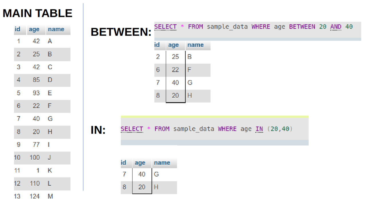
What is the meaning of selection bias and how to avoid it?
-
Sampling bias is the phenomenon that occurs when a research study design fails to collect a representative sample of a target population. This typically occurs because the selection criteria for respondents failed to capture a wide enough sampling frame to represent all viewpoints.
- The cause of sampling bias almost always owes to one of two conditions.
- Poor methodology: In most cases, non-representative samples pop up when researchers set improper parameters for survey research. The most accurate and repeatable sampling method is simple random sampling where a large number of respondents are chosen at random. When researchers stray from random sampling (also called probability sampling), they risk injecting their own selection bias into recruiting respondents.
- Poor execution: Sometimes data researchers craft scientifically sound sampling methods, but their work is undermined when field workers cut corners. By reverting to convenience sampling (where the only people studied are those who are easy to reach) or giving up on reaching non-responders, a field worker can jeopardize the careful methodology set up by data scientists.
- The best way to avoid sampling bias is to stick to probability-based sampling methods. These include simple random sampling, systematic sampling, cluster sampling, and stratified sampling. In these methodologies, respondents are only chosen through processes of random selection—even if they are sometimes sorted into demographic groups along the way.
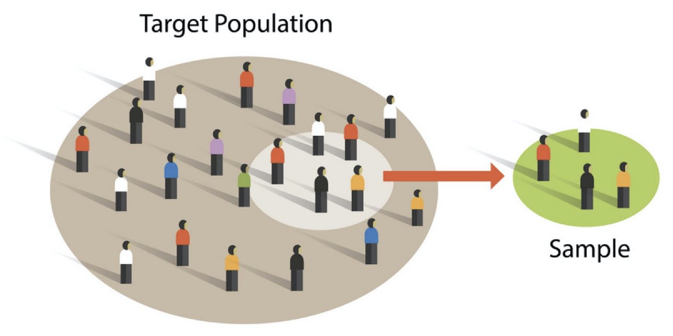
Given two python series, write a function to compute the euclidean distance between them?
- There are different ways to solve this question. The notebook snippet below shows various ways (along with credits to the respetive individual authors) and also shows the computation time for each method. Furthermore, the computation time for each method is calculated depending on whether the input was a NumPy array vs. Python Series and as shown using a NumPy array decreases the computation time.
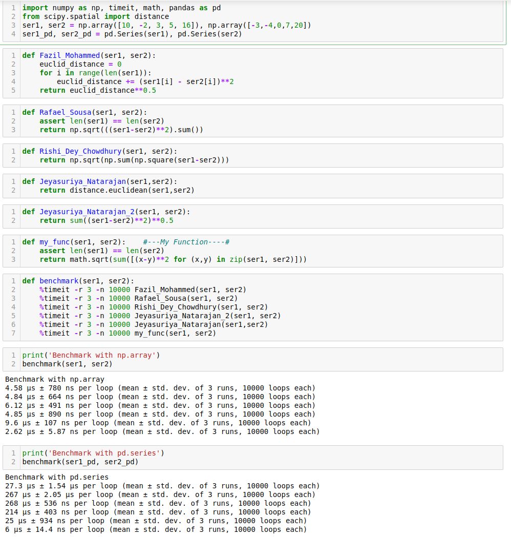
Define the cross-validation process and the motivation behind using it?
-
Cross-validation is a technique used to assess the performance of a learning model in several subsamples of training data. In general, we split the data into train and test sets where we use the training data to train our model and the test data to evaluate the performance of the model on unseen data and validation set for choosing the best hyperparameters. Now, a random split in most cases (for large datasets) is fine. But for smaller datasets, it is susceptible to loss of important information present in the data in which it was not trained. Hence, cross-validation though computationally bit expensive combats this issue.
-
The process of cross-validation is as the following:
- Define \(k\) or the number of folds.
- Randomly shuffle the data into \(k\) equally-sized blocks (folds).
- For each \(i\) in fold (1 to \(k\)), train the data using all the folds except for fold \(i\) and test on the fold \(i\).
- Average the \(k\) validation/test error from the previous step to get an estimate of the error.
- This process aims to accomplish the following:
- Prevent overfitting during training by avoiding training and testing on the same subset of the data points
- Avoid information loss by using a certain subset of the data for validation only. This is important for small datasets.
- Cross-validation is always good to be used for small datasets, and if used for large datasets the computational complexity will increase depending on the number of folds.
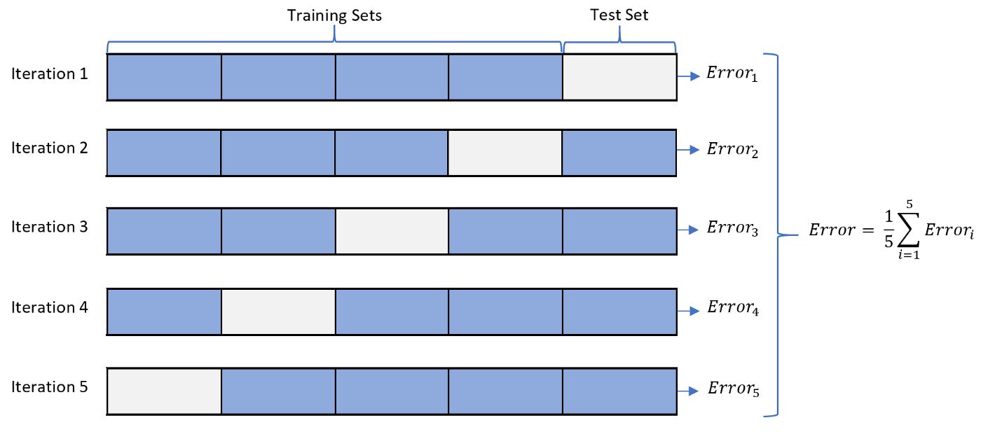
What is the difference between the Bernoulli and Binomial distribution?
- Bernoulli and Binomial are both types of probability distributions.
-
The function of Bernoulli is given by
\[p(x) =p^x * q^(1-x), x=[0,1]\]- where,
- Mean is \(p\).
- Variance \(p*(1-p)\).
- where,
-
The function Binomial is given by:
\[p(x) = nCx p^x q^(n-x) x=[0,1,2...n]\]- where,
- Mean: \(np\).
- Variance: \(npq\). Where p and q are the probability of success and probability of failure respectively, n is the number of independent trials and x is the number of successes.
- where,
- As we can see sample space (\(x\)) for Bernoulli distribution is Binary (2 outcomes), and just a single trial.
- For e.g., a loan sanction for a person can be either a success or a failure, with no other possibility. (Hence single trial).
- Whereas for Binomial the sample space (\(x\)) ranges from \(0-n\).
- As an example, tossing a coin 6 times, what is the probability of getting 2 or a few heads?
- Here sample space is \(x=[0,1,2]\) and more than 1 trial and \(n=6\) (finite).
- In short, Bernoulli Distribution is a single trial version of Binomial Distribution.
Given an integer \(n\) and an integer \(K\), output a list of all of the combinations of \(k\) numbers chosen from 1 to \(n\). For example, if \(n=3\) and \(k=2\), return \([1,2],[1,3],[2,3]\).
- There are different solutions one of them is the one below, there are other solutions in the comments of the original post and also the benchmarking between them thanks to Behnam Hedayat
from itertools import combinations
def find_combintaion(k, n):
	list_num = []
	comb = combinations([k for x in range (1, n+1)], k)
	for i in comb:
		list_num.append(i)

	print("(k: {}, n: {}):".format(k, n))
	print(list_num, "\n")
Explain the long-tailed distribution and provide three examples of relevant phenomena that have long tails. Why are they important in classification and regression problems?
- A long-tailed distribution is a type of heavy-tailed distribution that has a tail (or tails) that drop off gradually and asymptotically.
- Three examples of relevant phenomena that have long tails:
- Frequencies of languages spoken
- Population of cities
- Pageviews of articles
- All of these follow something close to the 80-20 rule: 80% of outcomes (or outputs) result from 20% of all causes (or inputs) for any given event. This 20% forms the long tail in the distribution.
- It’s important to be mindful of long-tailed distributions in classification and regression problems because the least frequently occurring values make up the majority of the population. This can ultimately change the way that you deal with outliers, and it also conflicts with some machine learning techniques with the assumption that the data is normally distributed.
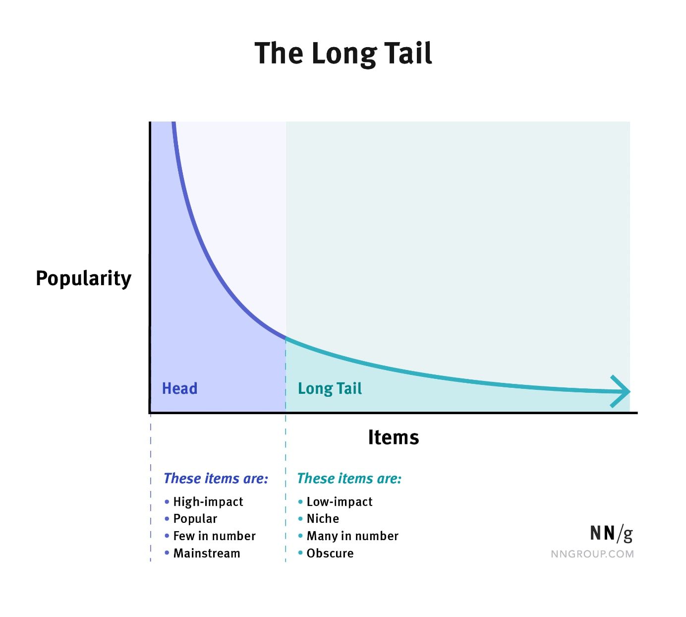
You are building a binary classifier and found that the data is imbalanced, what should you do to handle this situation?
- If there is a data imbalance there are several measures we can take to train a fairer binary classifier:
- Pre-Processing:
- Check whether you can get more data or not.
- Use sampling techniques (Up-sample minority class, downsample majority class, can take the hybrid approach as well). We can also use data augmentation to add more data points for the minority class but with little deviations/changes leading to new data points which are similar to the ones they are derived from. The most common/popular technique is SMOTE (Synthetic Minority Oversampling technique)
- Suppression: Though not recommended, we can drop off some features directly responsible for the imbalance.
- Learning Fair Representation: Projecting the training examples to a subspace or plane minimizes the data imbalance.
- Re-Weighting: We can assign some weights to each training example to reduce the imbalance in the data.
- In-Processing:
- Regularizaion: We can add score terms that measure the data imbalance in the loss function and therefore minimizing the loss function will also minimize the degree of imbalance with respect to the score chosen which also indirectly minimizes other metrics which measure the degree of data imbalance.
- Adversarial Debiasing: Here we use the adversarial notion to train the model where the discriminator tries to detect if there are signs of data imbalance in the predicted data by the generator and hence the generator learns to generate data that is less prone to imbalance.
- Post-Processing:
- Odds-Equalization: Here we try to equalize the odds for the classes w.r.t. the data is imbalanced for correct imbalance in the trained model. Usually, the F1 score is a good choice, if both precision and recall scores are important
- Choose appropriate performance metrics. For example, accuracy is not a correct metric to use when classes are imbalanced. Instead, use precision, recall, F1 score, and ROC curve.
- Pre-Processing:
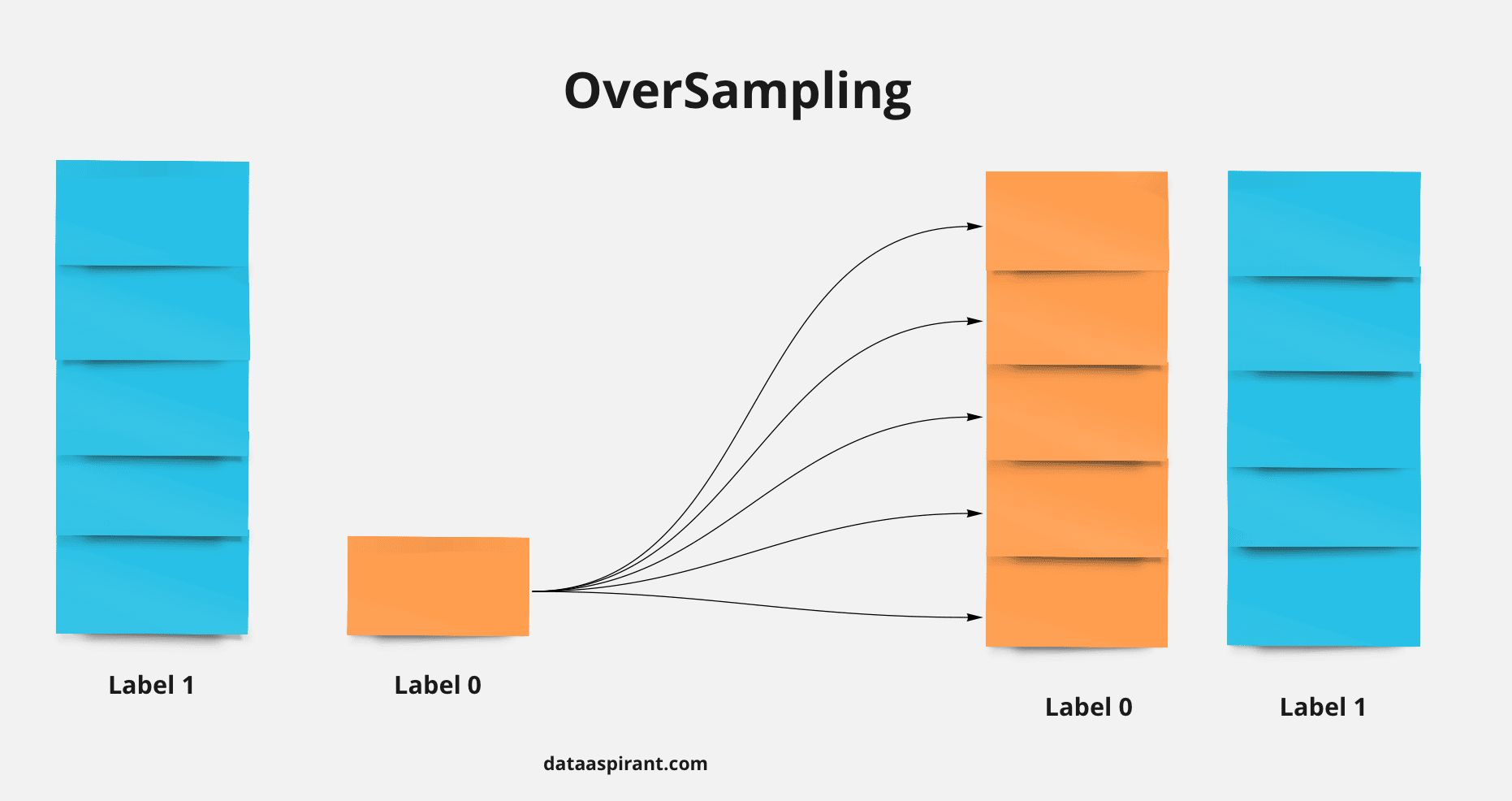
If there are 30 people in a room, what is the probability that everyone has different birthdays?
- The sample space is 365^30 and the number of events is \(365_p_30\) because we need to choose persons without replacement to get everyone to have a unique birthday therefore the Prob = \(365_p_30\) / 365^30 = 0.2936
- Interesting facts provided by Rishi Dey Chowdhury:
- With just 23 people there is over 50% chance of a birthday match and with 57 people the match probability exceeds 99%. One intuition to think of why with such a low number of people the probability of a match is so high. It’s because for a match we require a pair of people and 23 choose 2 is 23*11 = 253 which is a relatively big number and ya 50% sounds like a decent probability of a match for this case.
- Another interesting fact is if the assumption of equal probability of birthday of a person on any day out of 365 is violated and there is a non-equal probability of birthday of a person among days of the year then, it is even more likely to have a birthday match.
- A theoretical explanation is provided in the figure below thanks to Fazil Mohammed.
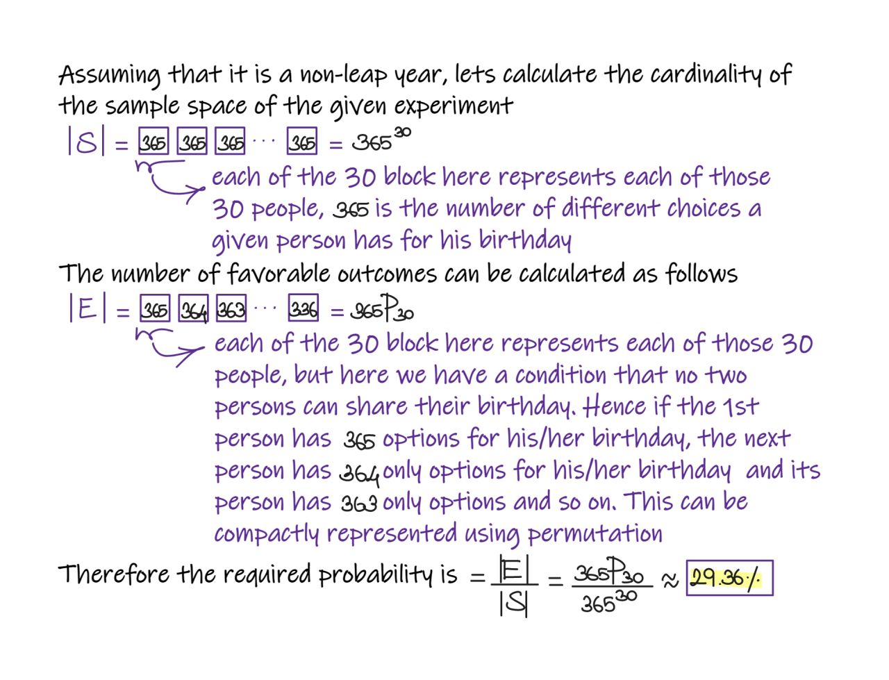
What is the Vanishing Gradient Problem and how do you fix it?
- The vanishing gradient problem is encountered in artificial neural networks with gradient-based learning methods and backpropagation. In these learning methods, each of the weights of the neural network receives an update proportional to the partial derivative of the error function with respect to the current weight in each iteration of training. Sometimes when gradients become vanishingly small, this prevents the weight to change value.
- When the neural network has many hidden layers, the gradients in the earlier layers will become very low as we multiply the derivatives of each layer. As a result, learning in the earlier layers becomes very slow. This can cause the network to stop learning. This problem of vanishing gradients happens when training neural networks with many layers because the gradient diminishes dramatically as it propagates backward through the network.
- Some ways to fix it are:
- Use skip/residual connections.
- Using ReLU or Leaky ReLU over sigmoid and tanh activation functions.
- Use models that help propagate gradients to earlier time steps such as GRUs and LSTMs.
What are Residual Networks? How do they help with vanishing gradients?
- Here is a concept that you should know whether you are trying to get a job in AI or you want to improve your knowledge of AI: residual networks.
- Skip connections or residual networks feed the output of a layer to the input of the subsequent layers, skipping intermediate operations.
- They appear in the Transformer architecture, which is the base of GPT4 and other language models, and in most computer vision networks.
- Residual connections have several advantages:
- They reduce the vanishing gradient since the gradient value is transferred through the network.
- They allow later layers to learn from features generated in the initial layers. Without the skip connection, that initial info would be lost.
- They help to maintain the gradient surface smooth and without too many saddle points.
- This keeps gradient descent to get stuck in local minima, in other words, the optimization process is more robust and then we can use deeper networks.
- ResNet paper was published at the end of 2015 and was very influential because, for the first time, a network with 152 layers surpassed the human performance in image classification.
- Deep learning is based on two competing forces: the more layers, the higher the generalization power of the network, however, the more layers, the more difficult is to optimize.
- In other words, the deeper the network, the better it models the real world in theory, however, it is very difficult to train in practice.
- ResNet was a very important step to solve this problem.
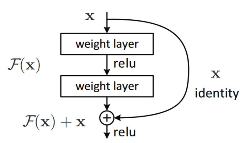
How does ResNet-50 solve the vanishing gradients problem of VGG-16?
- During the ImageNet Large Scale Visual Recognition Challenge (ILSVRC) that with the increase in the number of layers the deep learning models will perform better because of more parameters. However, because of more number of layers, there was a problem with vanishing gradients. In fact, the authors of ResNet, in the original paper, noticed that neural networks without residual connections don’t learn as well as ResNets, although they are using batch normalization, which, in theory, ensures that gradients should not vanish.
- Enter ResNet that utilize skip connections under-the-hood.
- The skip connections allow information to skip layers, so, in the forward pass, information from layer l can directly be fed into layer $l+t$ (i.e., the activations of layer $l$ are added to the activations of layer $l+t$, for $t >= 2$ and, during the forward pass, the gradients can also flow unchanged from layer $l+t$ to layer $l$. This prevents the vanishing gradient problem (VGP). Let’s explain how.
- The VGP occurs when the elements of the gradient (the partial derivatives with respect to the parameters of the network) become exponentially small, so that the update of the parameters with the gradient becomes almost insignificant (i.e., if you add a very small number $0 < \epsilon « 1$ to another number $d$, $d+\epsilon$ is almost the same as d and, consequently, the network learns very slowly or not at all (considering also numerical errors).
- Given that these partial derivatives are computed with the chain rule, this can easily occur, because you keep on multiplying small (finite-precision) numbers.
- The deeper the network, the more likely the VGP can occur. This should be quite intuitive if you are familiar with the chain rule and the back-propagation algorithm (i.e. the chain rule).
- By allowing information to skip layers, layer l+t receives information from both layer $l+t−1$ and layer $l$ (unchanged, i.e., you do not perform multiplications).
- From the paper: “Our results reveal one of the key characteristics that seem to enable the training of very deep networks: Residual networks avoid the vanishing gradient problem by introducing short paths which can carry gradient throughout the extent of very deep networks.”
How do you run a deep learning model efficiently on-device?
- Let’s take the example of LLaMA, a ChatGPT-like LLM by Meta.
- You can run one of the latest LLMs if you have a computer with 4Gb of RAM.
- The model is implemented in C++ (with Python wrappers) and uses several optimization techniques:
- Quantization
- Quantization represents the weights of the model in a low-precision data type like 4-bit integer (INT4) instead of the usual 32-bit floating precision (FP32).
- For example, the smallest LLaMA model has 7B parameters.
- The original model uses 13GB of RAM, while the optimized model uses 3.9GB.
- Faster weight loading
- Another optimization is to load the model weights using
mmap()instead of standard C++ I/O. - That enabled to load LLaMA 100x faster using half as much memory.
mmap()maps the read-only weights usingMAP_SHARED, which is the same technique that’s traditionally used for loading executable software.
- Another optimization is to load the model weights using
- Quantization
When are tress not useful?
- Use tree ensembles (random forest/gradient boosted trees) unless you have a reason not to.
- Here are some of the only reasons not to use tree ensembles for your supervised machine learning problem:
- You are working with unstructured data (text, image, audio, video)
- You are doing statistical inference on a parametric model to draw conclusions (for example, causal inference)
- You have strict interpretability requirements from a legal perspective
- You are trying to model a phenomenon with a known relationship in order to extrapolate the relationship (for example, logistic curves to model population growth scenarios)
- You have very restrictive latency and/or memory requirements (sparse linear models and SVMs are superior here)
- Ignoring these, tree ensembles are typically more adaptable and performant. Spend less time trying to beat them, and more time iterating on data quality, feature engineering, and MLOps best practices.
Misc
What is the difference between standardization and normalization?
- Normalization means rescaling the values into a range of (typically) [0,1].
- Standardization refers to centering the values around the mean with a unit standard deviation.
When do you standardize or normalize features?
- Rule of thumb:
- Standardization, when the data follows a Gaussian distribution and your algorithm assumes your data follows a Gaussian Distribution like Linear Regression.
- Normalization, when your data has varying scales and your algorithm doesn’t make assumptions about the distribution of your data like KNN.
Why is relying on the mean to make a business decision based on data statistics a problem?
- There is a famous joke in Statistics which says that, “if someone’s head is in the freezer and leg is in the oven, the average body temperature would be fine, but the person may not be alive”.
- Making decisions solely based on mean value is not advisable. The issue with mean is that it is affected significantly by the presence of outliers, and may not be the correct central representation of the dataset.
- It is thus advised that the mean should be used along with other measures and measures of variability for better understanding and explainability of the data.
Explain the advantages of the parquet data format and how you can achieve the best data compression with it?
-
The parquet format is something that every data person has to be aware about. Its a popular choice for data storage for faster query and better compression but do you know how the sorting order can be very important when we optimize for compression?
-
Parquet uses columnar storage, which means that data is stored by column rather than by row. This can lead to significant improvements in compression, because values in a column tend to be more homogeneous than values in a row. However, to achieve the best compression, it’s important to sort the data within each column in a specific way.
-
Parquet uses a technique called “run-length encoding” (RLE) to compress repetitive sequences of values within a column. RLE works by storing a value once, followed by a count of how many times that value is repeated. For example, if a column contains the values [1,1, 1, 1, 2, 2, 3, 3, 3, 3, 3], RLE would store it as [1, 4, 2, 2, 3, 5].
-
To take advantage of RLE, it’s important to sort the data within each column in a way that maximizes the number of repetitive sequences. For example, if a column contains the values [1, 2, 3, 4, 5, 1, 2, 3, 4, 5], sorting it as [1, 1, 2, 2, 3, 3, 4, 4, 5, 5] would result in better compression.
-
In addition to RLE, Parquet also uses other compression techniques such as dictionary encoding and bit-packing to achieve high compression ratios. These techniques also benefit from sorted data, as they can take advantage of the repetition and predictability of sorted values to achieve better compression.
-
What about the order of sorting when we sort on multiple columns, does that have an impact ? The asnwer is yes. Sorting the data by the most significant column(s) first can lead to better compression because it can group similar values together, allowing for better compression within each data page.
-
For example, consider a dataset with three columns: column1, column2 and column3. If most of the values in column1 are the same or similar (lower cardinality), then sorting the data by column1 first can help group together similar values and achieve better compression within each data page.
-
In summary, the sorting order of data can have a significant impact on data compression in Parquet and should be considered for data pipelines.
What is Redis?
- Redis is not just a key-value cache - it can be used as a database, as a pub-sub, and much more.
-
“Redis” actually stands for “Remote DIctionary Server”. Redis was originally designed as a key-value store database for remote access, with a focus on speed, simplicity, and versatility.
-
Since Redis’ code is open source, you can deploy Redis yourself. There are many ways of Redis deployment: standalone mode, cluster mode, sentinel mode, and replication mode.
-
In Redis, the most popular mode of deployment is cluster mode. Redis Cluster is a distributed implementation of Redis, in which data is partitioned and distributed across multiple nodes in a cluster.
-
In Redis Cluster, each node is responsible for a subset of the keyspace, and multiple nodes work together to form a distributed system that can handle large amounts of data and high traffic loads. The partitioning of data is based on hashing of the key, and each node is responsible for a range of hash slots.
-
The hash slot range is distributed evenly among the nodes in the cluster, and each node is responsible for storing and serving data for the hash slots assigned to it. When a client sends a request to a node, the node checks the hash slot of the requested key, and if the slot is owned by the node, the request is processed locally. Otherwise, the request is forwarded to the node that owns the slot.
-
Redis Cluster also provides features for node failover, in which if a node fails, its hash slot range is automatically taken over by another node in the cluster. This ensures high availability and fault tolerance in the system.
- Overall, in clustered Redis, data is arranged based on a consistent hashing algorithm, where each node is responsible for a subset of the keyspace and works together to form a distributed system that can handle large amounts of data and traffic loads.
References
- Why is it bad idea to initialize all weight to same value?
- Why doesn’t backpropagation work when you initialize the weights the same value?
- What is convergence in k-means?
- Clearly explained: Pearson v/s Spearman Correlation Coefficient
- How to choose between Pearson and Spearman correlation?
- Aman Prabhakar on LinkedIn
Citation
If you found our work useful, please cite it as:
@article{Chadha2020DistilledInterviewQuestions,
  title   = {Interview Questions},
  author  = {Chadha, Aman},
  journal = {Distilled AI},
  year    = {2020},
  note    = {\url{https://aman.ai}}
}