Left to Right
- Overview
- Data
- Features
- Metrics
- Embeddings
- Here is the requested information filled in:
- Loss/ Regularization/ Optimizer
- Retrieval: ANN
- Bloom Filter
- First Ranking LTR:
- Re Ranking
- Evaluation- before deploying
- Privacy: Differential Privacy
- Content Moderation: removal of toxicity
- Data Drift
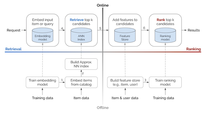
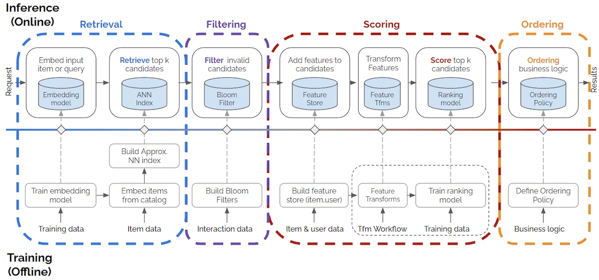
Overview
Data
- User item logs are stored in S3
- Should have implicit and explicit signals here
User ID	Item ID	Timestamp	Action Type	Action Value
1	101	2023-07-08 08:45	viewed	N/A
2	102	2023-07-08 09:15	purchased	N/A
1	103	2023-07-08 10:30	rated	4.5
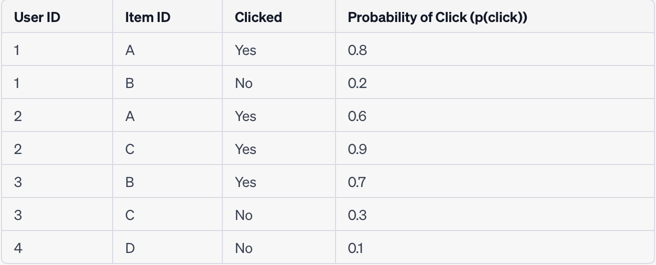
- Data for user-item interaction can vary depending on the specific goals and hypotheses of the recommender system. If the objective is to predict the probability of a click (p(click)), the data can be structured as follows:
| User ID | Item ID | Clicked |
|---|---|---|
| 1 | A | Yes |
| 1 | B | No |
| 2 | A | Yes |
| 2 | C | Yes |
| 3 | B | Yes |
| 3 | C | No |
| 4 | D | No |
- Amazon Athena to extract features from S3 data
- Take this data and convert to matrix via np.matrix() and give it as input to SVD or ALS
Features
- Feature engineering is the process of leveraging prior knowledge of the raw data and representing it in a manner that better facilitates learning.
- Robusta: in house feature platform
- User-related features:
- Demographic information: Age, gender, location, language, etc.
- User history: User’s viewing history, previously watched videos, liked or disliked videos, and user feedback (ratings, comments, shares).
- User preferences: User-selected genres, topics, or categories of interest.
- User behavior: Time spent on videos, frequency of video interactions, session duration, click-through rate, watch time, etc.
- Social connections: Social network information, friends’ preferences, or recommendations based on social interactions.
- Item-related features:
- Metadata: Title, description, tags, genres, release date, duration, language, etc.
- Content-based features: Audio analysis, video visual features (e.g., color, composition), text analysis of subtitles or transcripts, video length, visual similarity to other videos, etc.
- Popularity indicators: Number of views, likes, shares, comments, trending status, etc.
- Categorization: Genres, topics, subcategories, or tags associated with the video.
- Collaborative filtering: Similarity measures based on user-item interactions, such as user-item ratings or item co-occurrence.
- In the context of a recommender system, features can come in a variety of forms. The nature of these features will often depend on the specifics of the content being recommended, the available user data, and the specific objectives and strategies of the recommender system. Below are some examples of what these features might look like:
User-specific features:
- User Demographics: Age, gender, location, language preference, etc.
- User Behavior: Browsing history, transaction history, click-through rates, watch time, viewing patterns, feedback/ratings, frequency and duration of sessions, etc.
Content-specific features:
- Content Metadata: For a video recommender system, for instance, this could be the video title, length, genre, language, release date, actors/directors, etc.
- Content Description: A textual description or summary of the content.
- Content Popularity: The number of views, likes, shares, or comments on the content.
Interaction features:
- Previous Interactions: Whether the user has previously interacted with the content (e.g., viewed, liked, shared, rated, etc.), and the nature of those interactions (e.g., length of view, positive or negative rating, etc.).
- Related Interactions: Whether the user has interacted with similar content (e.g., content in the same genre, from the same creator, etc.), and the nature of those interactions.
Contextual features:
- Time-based Context: Time of the day, day of the week, season of the year, etc.
- Device Context: Whether the user is using a desktop, laptop, smartphone, tablet, etc.
-
Each of these features would generally be represented numerically, so they can be processed by a machine learning model. For instance, categorical features like gender or genre could be one-hot encoded or embedded into a lower-dimensional space, and textual features could be transformed into a numerical representation using techniques like TF-IDF or word embeddings. Temporal features might be represented as a cyclic encoding to capture the periodic nature of time.
- User Features:
- user_id: Unique identifier for each user
- user_age: Age of the user
- user_gender: Gender of the user
- user_location: Location of the user
- user_history: Past videos watched by the user
- Video Features:
- video_id: Unique identifier for each video
- video_length: Duration of the video
- video_genre: Genre of the video (e.g., Comedy, Drama, etc.)
- video_director: Director of the video
- video_actors: List of main actors in the video
- Interaction Features:
- watched: Whether the user watched the video (binary)
- rating: Rating given by the user to the video (if available)
- watch_time: How long the user watched the video
Metrics
For a video recommender problem, you can use both offline and online metrics to evaluate the performance of your recommendation system.
Offline metrics assess the quality of recommendations using historical data and do not require user feedback during the evaluation process. These metrics provide insights into how well the model performs based on past data. Some commonly used offline metrics for video recommendation systems include:
-
Precision at K (P@K): This metric measures the proportion of recommended videos in the top K positions that are relevant to the user. It calculates the precision of the recommendations among the top K items.
-
Recall at K (R@K): This metric measures the proportion of relevant videos among the top K recommended videos. It captures the ability of the system to retrieve relevant videos from the entire pool of possible recommendations.
-
Mean Average Precision at K (MAP@K): This metric computes the average precision at each position up to K and takes the mean. It considers the order of the recommendations and provides a more comprehensive evaluation of the system’s performance.
-
Normalized Discounted Cumulative Gain (NDCG): NDCG measures the quality of the recommended videos based on their relevance and position in the list. It assigns higher scores to relevant videos appearing at the top positions.
While offline metrics provide insights into recommendation quality based on historical data, they have limitations as they do not consider real-time user feedback or account for the actual impact of recommendations on user satisfaction. Therefore, online metrics are essential to measure the performance of the recommendation system in real-world scenarios.
Online metrics evaluate the performance of the recommendation system based on user interactions and feedback in a live environment. These metrics capture user engagement, click-through rates, and other relevant user actions. Some common online metrics for video recommender systems include:
-
Click-Through Rate (CTR): CTR measures the proportion of users who click on the recommended videos out of the total number of impressions. It indicates the effectiveness of the recommendations in attracting user attention.
-
Conversion Rate: Conversion rate measures the proportion of users who perform a desired action (e.g., watching a video, subscribing, or liking) after being recommended a video. It evaluates the ability of the system to drive user engagement.
-
View Time: View time measures the total duration of video views generated by the recommendations. It provides insights into the system’s ability to recommend videos that capture users’ interest and keep them engaged.
-
User Engagement: User engagement metrics evaluate user behavior after consuming the recommended videos, such as likes, comments, shares, or subscriptions. They reflect the impact of recommendations on user satisfaction and interaction.
- It is important to analyze both offline and online metrics together to gain a comprehensive understanding of the performance and impact of the video recommender system. Offline metrics provide insights into recommendation quality, while online metrics reflect real-world user behavior and satisfaction.
Embeddings
- Matrix Factorization (MF):
- Use it when you’re dealing with explicit user-item interaction data (e.g., ratings).
- Computationally efficient, easy to implement, and easy to interpret, which makes it a good starting point for any recommendation system.
- However, it only captures linear relationships and ignores other potentially valuable information like content features and temporal dynamics.
- Neural Collaborative Filtering (NCF):
- Use it when you want to capture complex, non-linear relationships in your data.
- It works well with both explicit (e.g., ratings) and implicit feedback (e.g., clicks, purchase history).
- However, it can be computationally intensive and harder to interpret.
- Two-Tower Models:
- Use it when you have a large catalog of items and need to perform efficient retrieval of the top-N items for a user.
- It’s useful when you have rich feature data (both for users and items), as you can feed these features into the respective towers.
- It allows you to perform large-scale recommendation tasks efficiently by using approximate nearest neighbor (ANN) techniques.
- However, these models can be complex to set up and require more computational resources.
Matrix Factorization
- Loss function is MSE(difference between observed and predicted value):
- It’s used to approximate the original user-item interaction matrix that it takes as input and output user and item embeddings via ALS
- ALS captures the underlying patterns and interactions between users and items. It offers a scalable and parallelizable approach to factorization, making it suitable for large-scale recommendation systems.
Neural Collaborative Filtering Framework
- The input data for NCF typically involves positive and negative training samples.
- User ID Encoding: {“User1”: [0.2, 0.4, 0.1], “User2”: [0.3, 0.1, 0.5], “User3”: [0.6, 0.2, 0.3], “User4”: [0.1, 0.6, 0.4]}
-
Item ID Encoding: {“Item1”: [0.7, 0.4, 0.2], “Item2”: [0.9, 0.5, 0.1], “Item3”: [0.3, 0.8, 0.6]}
- Implemented by below:
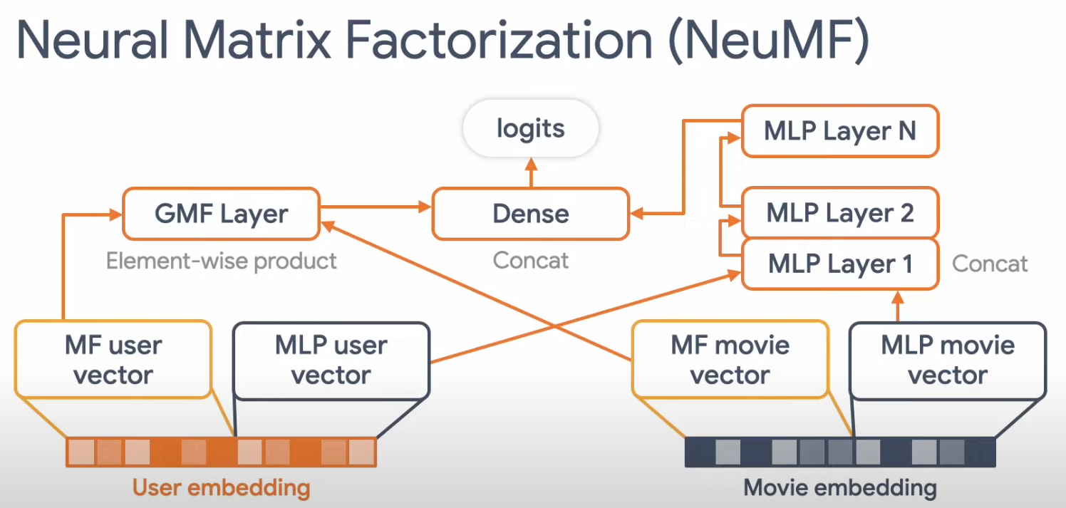
Neural Matrix Factorization
- Input: The input to NeuMF is typically a sparse user-item interaction matrix, where each cell represents the interaction strength (e.g., the rating that a user has given to an item). Additionally, user and item metadata can also be incorporated.
User ID	Item ID	Interaction Strength
User1	Item1	5.0
User1	Item2	4.0
User2	Item1	3.0
- Output: The output from NeuMF is a set of dense vectors, one for each user and one for each item. These vectors (embeddings) capture the latent factors of the users and items. During the candidate generation phase, these vectors can be used to compute a similarity score between a user and each item, and the items with the highest scores would be output as the candidate items for that user.
User1: [0.1, -0.3, 0.4, ...] Item1: [0.2, 0.1, -0.5, ...] - It is an ensemble of Generalized Matrix Factorization (GMF) and a Multi-Layer Perceptron (MLP)
- Takes the Matrix Factorization user and item embedding and replaces the inner product with a MLP that can learn the distribution/arbitrary function from data.
- Generalized Matrix Factorization (GMF): This takes the approach of traditional matrix factorization but introduces non-linearities.
- Multi-Layer Perceptron (MLP): This is a more flexible model that concatenates (rather than dot-products) the user and item embeddings, and then passes them through multiple fully-connected layers to learn the interaction between user and item embeddings.
- They concatenate the last hidden layer
- hybrid
- You can add another parallel pathway to the existing Generalized Matrix Factorization (GMF) and Multi-Layer Perceptron (MLP) pathways to process content-based features. This pathway could be an MLP that takes content-based features as input and outputs an embedding. This new embedding is then concatenated with the GMF and MLP embeddings before the final prediction layer.
Two Towers
- Input: The input for a two-tower model could be user and item features, such as user demographics, item characteristics, and historical interaction data. These features could be either categorical or numerical, and they would be transformed into dense vectors (embeddings) through an embedding layer in the model.
User ID	Feature1	Feature2	...
User1	Value1	Value2	...
User2	Value3	Value4	...
...	...	...

Item ID	Feature1	Feature2	...
Item1	Value1	Value2	...
Item2	Value3	Value4
- Output: Like NeuMF, the output from a two-tower model is a set of dense vectors for the users and items. These vectors are then used to compute similarity scores for candidate generation.
For each user and item, a dense vector is generated, representing their latent factors.
User1: [0.1, -0.3, 0.4, ...]
Item1: [0.2, 0.1, -0.5, ...]
- Embedding based retrieval:
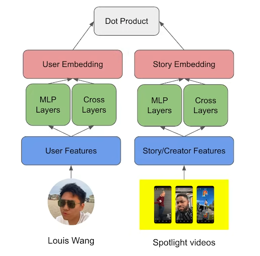
- ResNet: The ResNet-style structure helps deal with the problem of vanishing gradients that can occur in deep networks. It allows the model to learn from large amounts of data more effectively by using skip connections or shortcuts.
- MLP (Multi-Layer Perceptron): MLPs are powerful tools for processing complex patterns in the data. By passing the features through an MLP, the model is able to transform the original features into a higher-level feature space where they can be more easily separated.
- Deep Cross Network: The deep cross network helps with learning high-order feature interactions. This means it’s capable of understanding complex relationships between different features, which can be crucial in generating high-quality embeddings.
- The embeddings themselves are a compact representation of the input data and these layers help in creating these embeddings that capture the essential aspects of the data in lower dimensions. The aim is to create embeddings that encapsulate as much useful information as possible from the input features. The combination of these layers allows the model to learn more complex representations and interactions, improving its predictive power.
- However, there is always a trade-off between complexity and interpretability in machine learning models. More complex models like this one can provide better performance, but they can also be harder to understand and potentially overfit if not properly regularized or if they are used with insufficient amounts of data. It’s crucial to consider these factors when designing a machine learning architecture.
- hybrid: In the item tower, you can process both collaborative filtering information and content-based features. The content-based features can be incorporated into the item embeddings, for example, by concatenating the content-based and collaborative filtering embeddings, or by passing them through a shared layer.
Deep Cross Network
- Input: The input to a DCN is typically a set of categorical and/or numerical features, such as user demographics and item characteristics. These features are transformed into dense vectors via an embedding layer for categorical features and a normalization layer for numerical features.
User ID Item ID Feature1 Feature2 ... User1 Item1 Value1 Value2 ... User1 Item2 Value3 Value4 ... User2 Item1 Value5 Value6 - Output: The output from a DCN can be a prediction score that quantifies the interaction strength between a user and an item. For candidate generation, you would compute the scores for a user-item pair and select the items with the highest scores as the candidates.
A prediction score for each user-item pair.
hybrid: DCN can process high-dimensional sparse features as well as dense features. Thus, you can input content-based features into the DCN along with the collaborative filtering features. The DCN will learn complex interactions between these different types of features.
Non personalized recommendations for User cold start
- Have rule based, where after 10 interactions we switch out of popularity model
Wide and Deep
- Input: Similar to DCN, the input for a Wide & Deep model consists of both wide (sparse, categorical) and deep (dense, numerical) features. Wide features might include cross-product feature transformations, while deep features might include user and item embeddings.
-
Output: The Wide & Deep model also outputs a prediction score for a user-item pair, which can be used for candidate generation by selecting the items with the highest scores for each user.
- hybrid: Content-based features can be included in both the wide and the deep parts of the model. In the wide part, you can define cross-product feature transformations between user and item features to capture their interactions. In the deep part, you can include user and item features as inputs to the feed-forward neural network. The deep part can learn complex interactions among all the features.
Content based
- BM25 (Best Match 25): BM25 is a ranking function that measures the relevance of a document (item) with respect to a query (user). It takes into account factors such as term frequency, inverse document frequency, and document length normalization. BM25 assigns higher weights to terms that are rare in the entire document collection but frequent within a specific document. It is often used for search engines and information retrieval tasks. In the context of content-based filtering, BM25 can be used to calculate the similarity between user profiles (queries) and item features (documents) and generate content-based embeddings based on the relevance scores.
- TF-IDF (Term Frequency-Inverse Document Frequency): TF-IDF is a statistical measure that reflects the importance of a term in a document corpus. It considers both the frequency of a term in a document (term frequency) and the rarity of the term across the entire corpus (inverse document frequency). TF-IDF assigns higher weights to terms that are more frequent within a document but less frequent in the entire corpus. It is commonly used for information retrieval and text mining tasks. In content-based filtering, TF-IDF can be used to calculate the importance or relevance of terms within item descriptions, titles, or other text features. The TF-IDF scores can be used as the basis for creating content-based embeddings.
- word embeddings
- Both BM25 and TF-IDF are effective methods for capturing the importance of terms within the text-based features of items. They can be used to represent the content of items as feature vectors or embeddings, which can then be compared or used for similarity calculations in content-based recommendation systems. The choice between BM25 and TF-IDF depends on the specific requirements of the system and the characteristics of the text data being processed.
LLM (Language Model):
- LLM refers to a language model used in recommender systems, typically based on models like BERT (Bidirectional Encoder Representations from Transformers). BERT is a pre-trained language model that learns contextualized word representations by leveraging a large amount of unlabeled text data.
- In the context of a recommender system, LLM-based embeddings can be utilized to capture semantic relationships between items, user preferences, or contextual information from user reviews or item descriptions. These embeddings can provide a better understanding of the textual content associated with items or user interactions.
GNN (Graph Neural Network):
- GNN stands for Graph Neural Network, which can be used for embedding generation in recommender systems. Specifically, entity embeddings are commonly employed in GNN-based recommender systems.
- Entity embeddings in GNN-based recommender systems represent users, items, or other entities as low-dimensional vectors in a graph structure. GNNs process the graph data by propagating information through the network, allowing for capturing the relationships and interactions between entities.
- The entity embeddings obtained from GNNs enable the modeling of complex user-item interactions, taking into account the network structure and relational dependencies in the recommender system. These embeddings can be used to generate personalized recommendations based on the learned representations and the graph connectivity information.
Here is the requested information filled in:
Loss/ Regularization/ Optimizer
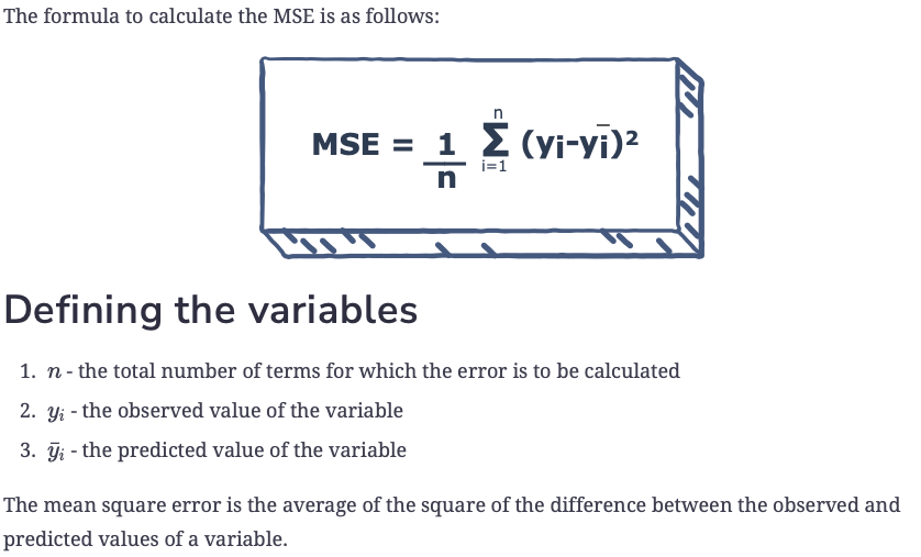
- Mean Square Error
- Mean Square Error (MSE) is a popular loss function commonly used in regression problems. It measures the average of the squares of the errors—that is, the average squared difference between the predicted and actual values. The mathematical expression is:
- MSE = (1/n) * Σ(actual value - prediction)^2
-
This function penalizes larger errors more due to the squaring operation, causing the model to prioritize reducing larger errors.
- Mean Absolute Error
- Mean Absolute Error (MAE) is another loss function typically used in regression problems. It measures the average magnitude of errors in a set of predictions, without considering their direction. The mathematical expression is:
-
MAE = (1/n) * Σ actual value - prediction -
This function is less sensitive to outliers compared to MSE because it does not square the error values, making it suitable for certain scenarios where we don’t want to significantly penalize larger errors.
- L1 or L2 Regularization
- Regularization is a technique to prevent overfitting in a model by adding a penalty term to the loss function.
- L1 regularization, also known as Lasso Regression, adds an L1 penalty equal to the absolute value of the magnitude of the coefficients. It tends to produce sparse solutions, pushing some coefficient estimates to be exactly zero.
-
L2 regularization, also known as Ridge Regression, adds an L2 penalty equal to the square of the magnitude of the coefficients. This typically results in smaller coefficient estimates. Unlike L1 regularization, L2 regularization does not force coefficients to zero, hence, doesn’t result in a sparse solution.
- Adam Optimizer
- Adam (Adaptive Moment Estimation) is an optimization algorithm that can be used instead of the classical stochastic gradient descent to update network weights iteratively based on training data. Adam combines the best properties of two other popular optimizers, AdaGrad and RMSProp. Adam adapts the learning rate for each parameter, helping the model to converge faster. This is done by calculating an exponential moving average of the gradient and the squared gradient, and the parameters beta1 and beta2 control the decay rates of these moving averages.
Retrieval: ANN
-
ANN (Approximate Nearest Neighbor) methods are used for efficient retrieval of nearest neighbors or similar items/users from a large dataset. Here’s a general overview of how ANN works:
- Input:
- Dataset: ANN methods take a dataset containing embeddings or similarity scores as input. These embeddings can represent users, items, or any other entities in the recommendation system. The embeddings capture the relevant features or characteristics of the entities.
- The input to ANN is a set of vectors. In a recommender system, each vector represents a user or item embedding. These embeddings are multi-dimensional, and each dimension captures some latent features of the user or item. They are usually generated using methods such as matrix factorization or deep learning.
- Query: In the context of recommendation, the query is typically a user or an item for which we want to find the most similar neighbors or items.
- Output:
-
The output of ANN methods is a set of nearest neighbors or similar items/users based on the provided query. The output can be a ranked list of items or a subset of the dataset that is considered most similar to the query.
- Indexing:
- Once we have the embeddings, the next step is to create an efficient data structure, also known as an index, that can facilitate fast retrieval of similar vectors.
- The goal here is to organize the embeddings in such a way that reduces the need to perform computations with all embeddings when a query comes in.
- This is a preprocessing step, and different ANN libraries (like HNSW, FAISS, SCANN, ANNOY) use different methods to create these indices.
- ANN implementations:
- Locality-Sensitive Hashing (LSH): Locality-Sensitive Hashing (LSH) is a method of performing probabilistic dimension reduction of high-dimensional data. The key idea of LSH is to hash the input items so that similar items are mapped to the same “buckets” with high probability (the number of buckets being much smaller than the universe of possible input items). LSH hashes input items several times in such a way that similar items are more likely to end up in the same hash bucket. This makes it possible to limit the search of nearest neighbors to the items that hash to the same bucket, reducing the search space drastically.
- Hierarchical Navigable Small World (HNSW): HNSW constructs a hierarchical graph where each layer is a navigable small world graph. It allows for very efficient ANN searches because at higher layers, the graph is sparse and thus you can make large “jumps” across the data, while the lower layers allow for refinement of the search. This hierarchical organization leads to logarithmic search complexity, providing very fast, yet precise search capabilities.
- KD-tree: KD-tree is a binary search tree where data in each node is a K-dimensional point in space. It is used to partition the space into regions, so that we can eliminate many points at once, making the search process faster. Points to the left of the plane are contained in the left subtree of that node and points to the right of the plane are contained in the right subtree. This rule applies recursively, such that for any node in the tree, all the nodes in the left subtree are to the left of the plane, and all nodes in the right subtree are to the right. While it works well in lower dimensions, KD-tree is not efficient for high-dimensional data due to the curse of dimensionality.
- Query: Now let’s say a user interacts with your service, and you want to provide some recommendations. You would first translate this user into a query vector. This could be the user’s embedding, or the embedding of an item they’ve interacted with.
- Retrieval: Using the query vector, the ANN method will refer to the index and quickly retrieve a list of vectors that are nearest to the query vector. The notion of “nearness” is often defined by a measure of distance in the embedding space, such as Euclidean distance or cosine similarity.
- Output: The retrieved vectors represent the items that you will recommend to the user. They can be returned in a ranked list, where the items that have the shortest distance to the query vector are ranked higher.
Bloom Filter
- Filter invalid candidates
- Bloom filter can be used to filter out invalid candidates by storing the information about items that are known to be invalid. Here’s how you can apply a Bloom filter for this purpose:
- Identify invalid candidates: Determine the criteria for identifying invalid candidates. For example, you may have certain videos that are flagged as inappropriate, expired, or violate community guidelines.
- Create a Bloom filter: Initialize a Bloom filter data structure with an appropriate size and number of hash functions. The size and number of hash functions should be chosen based on the expected number of items to be filtered and the desired false positive rate.
- Populate the Bloom filter: For each identified invalid candidate, add its unique identifier (e.g., video ID) to the Bloom filter. This is typically done during the data preprocessing or update phase of the recommender system.
- Filter candidates using the Bloom filter: During the candidate generation phase, retrieve a set of potential candidates for a given user. Before performing any further computations or analysis on these candidates, check each candidate’s unique identifier against the Bloom filter. If the identifier is not present in the Bloom filter, it is highly likely to be a valid candidate. However, if the identifier is found in the Bloom filter, it is considered invalid and can be filtered out without any further processing.
- By using a Bloom filter, you can efficiently eliminate a large portion of invalid candidates early in the recommendation pipeline, saving computational resources and improving the overall efficiency of the system. It provides a quick and memory-efficient way to identify potential invalid candidates based on their unique identifiers without the need for expensive operations, such as database queries or complex filtering criteria.
- pybloom-live and bitarray that can be used to implement a Bloom filter.
First Ranking LTR:
- Pointwise: In a pointwise approach, each item is considered in isolation without regard to other items. This is the simplest approach, treating the ranking problem as a regression or classification problem. In the case of video recommendation, each video will be scored independently based on its features and the user’s features. The videos are then ranked based on their scores.
- Linear regression: This is the most straightforward application of pointwise approach, where we predict a score for each item independently.
- Logistic Regression/ Classification models: The problem can be modeled as a binary or multi-class classification where classes represent different “ranking levels” of the items.
- Neural Networks: These can be used to capture non-linearities in the data and complex interactions between features. They can be used to predict scores for items independently.
- Pairwise: In the pairwise approach, the idea is to take a pair of items and design a binary classifier that can tell which item is better. This approach models the relative order between items and does not directly optimize the ranking list. In the context of video recommendation, this would mean comparing pairs of videos for a given user and deciding which one is preferred. The ranking is based on the number of wins an item gets when compared pairwise.
- RankNet: A model proposed by Microsoft Research, which is a pairwise LTR model using a neural network to model the ranking function.
- Support Vector Machines for Ranking (RankSVM): This pairwise model uses the concept of support vector machines to rank items.
- Listwise: The listwise approach models the entire list of items. It takes into consideration the interactions between items and attempts to optimize the ordering of the entire list of items directly. In video recommendation, this approach would take into account the entire list of videos and rank them in an order that would optimize a certain metric (like click-through rate, watch time, etc.).
- ListNet: This model uses a neural network and transforms the ranking problem into a problem of minimizing the loss of listwise probability.
- LambdaMART / LambdaRank: These are listwise approaches based on decision trees and boosting algorithms. LambdaMART is the boosted tree version of LambdaRank, which was based on RankNet. LambdaMART is known for being the winning algorithm of Yahoo’s 2010 Learning to Rank Challenge.
- ListMLE: This is another listwise method that employs maximum likelihood estimation for optimization.
Re Ranking
- Diversity:
- Diversity in recommendations is often pursued to prevent over-specialization and to ensure a broad range of content is shown to the user.
- This can be achieved by using Multi-Objective Optimization (MOO). For example, one objective can be to maximize relevance while another objective can be to maximize diversity in the recommended list of items.
- The trade-off between these objectives can be controlled by assigning appropriate weights to each objective.
- Business Rules:
- Business rules can be incorporated into the recommendation system in a number of ways.
- These rules could specify constraints (for example, certain videos should not be recommended to certain user groups) or priorities (e.g., newly released videos should be recommended more frequently).
- Multi-Armed Bandits (MAB) can be used to introduce such rules as part of the reward function. For instance, recommending a newly released video could yield a higher reward.
- Personalization:
- Personalization in a recommendation system is about tailoring the recommendations to the specific preferences and needs of the user.
- Contextual Bandits are particularly useful for personalization. They take into account the current context (like user’s demographic, recent activity, time of day, etc.) when making recommendations.
- Ensemble of Contextual bandits for ever changing user interest
- Fairness (less popular also gets an equal shot):
- Fairness in recommendation systems can refer to giving equal opportunity to items that are less popular or new and have less data.
- This can be addressed by using Multi-Armed Bandits (MAB). MAB strategies, especially those with an exploration component (like ε-greedy or Upper Confidence Bound (UCB)), can help ensure that less popular items are also shown to users.
- These techniques balance the trade-off between exploration (trying out less popular items) and exploitation (recommending items that are known to be popular).
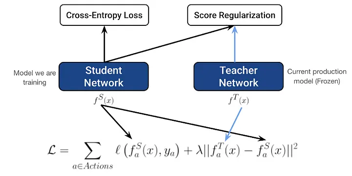
Score regularization
- To address model instability and ensure consistent ranking order, score regularization is introduced.
- This regularization technique aims to stabilize the predictions by distilling knowledge from a teacher model (the previous production model).
- During the training of the student model, the inference for the teacher model is performed, and a regularization term is added to the total loss. The coefficient 𝜆 is tuned to control the weight of this regularization term, which helps in achieving a more stable and consistent distribution of model predictions.
- The formulation of the score regularization is shown in Figure 3.
Evaluation- before deploying
- Evaluation is typically done using held-out validation or test data that were not used during training.
- Online:
- A/B testing, engagement, business rules
- Offline:
- Accuracy, Recall, precision, F1 score, NDCG
Privacy: Differential Privacy
- Differential privacy can be used to add a level of noise to the data to ensure that individual user data can’t be identified.
- This can be especially useful when dealing with sensitive data or to comply with regulations like GDPR.
- It helps to provide a balance between delivering personalized recommendations and preserving user privacy.
Content Moderation: removal of toxicity
Data Drift
- Guardrail metrics:
- Guardrail metrics: Guardrail metrics are predefined thresholds or performance indicators that help monitor the system’s performance and detect any significant deviations from the expected behavior. By continuously monitoring these metrics, you can identify potential data drift and take appropriate actions to adapt the recommendation algorithms or system configurations accordingly.
- Challenger Champion method - Continuous learning-
- The Challenger Champion method involves running multiple models concurrently in production. The champion model serves recommendations to users while the challenger model trains on new data in the background. Over time, as the challenger model demonstrates better performance and adapts to the data drift, it can be promoted to become the new champion. This approach allows for continuous learning and adaptation to changing user preferences and item popularity.
- Online learning-
- Online learning techniques enable the recommender system to adapt in real-time by updating the model based on incoming data. With online learning, the model can be updated incrementally as new data becomes available, allowing it to adapt to data drift. This ensures that the recommendations remain relevant and reflect the most up-to-date user preferences.