Applied Machine Learning for Industry

• Chapter Goals:
• TensorFlow protocol buffer
• Features
• Bytes and text
• Time to Code!
• TFRecords
  • Serialization
  • Writing to data files
  • Features
  • Example spec
  • VarLenFeature class
• FixedLenFeature class
  • Class configuration
• Parsing
• Input pipeline
• Image file dataset
• Specialized datasets
• Mapping function
• Wrapper functions
• Shuffling
• Epochs
• Batching
• Iterator
• Running the iteration
• Feature columns
• Categorical features
• Indicator wrapping
• Time to Code!
• Model Execution
  • Creating a model
• Training visualizations
• Tracking values
• Time to Code!
• Logging values
• Catching NaN
• Efficient training
• Checkpoints
• Model code
• Checkpoint directory
• Saving parameters
• Restoring parameters
• Training vs. evaluation
• Evaluation metrics
• Time to Code!
• Save For Inference
  • Deploying a model
  • Inference graph
  • Saving the model
  • Time to Code!
• Predictions
  • Restoring the model
  • Retrieving tensors
• Time to Code!
• Regression
  • Classification vs. regression
  • L2 loss
  • Time to Code!

Chapter Goals:

• Learn how protocol buffers are used in TensorFlow
• Implement a function to convert a Python dictionary to a tf.train.Example object

TensorFlow protocol buffer

• Since protocol buffers use a structured format when storing data, they can be represented with Python classes. In TensorFlow, the tf.train.Example class represents the protocol buffer used to store data for the input pipeline.
• Each individual tf.train.Example object describes data for a single dataset observation (e.g. a single row in a data table). We convert raw data to a protocol buffer by initializing a tf.train.Example object with the data’s values.
• When we initialize a tf.train.Example object, we need to set that object’s features argument to a tf.train.Features object. The tf.train.Features class is initialized by setting the feature field to a dictionary that maps feature names to feature values.

import tensorflow as tf

features = tf.train.Features(feature=f_dict)  # f_dict is a dict
ex = tf.train.Example(features=features)
print(repr(ex))

• The code above initializes a tf.train.Example object. Note that f_dict is a dictionary mapping feature names to feature values. We discuss how to create the feature dictionary later in this chapter.

Features

• Each feature value is represented by a tf.train.Featur object, which is initialized with exactly one of the following fields:
  • int64_list, for integer data values. Set with a tf.train.Int64List object.
  • float_list, for floating point data values. Set with a tf.train.FloatList object.
  • bytes_list, for byte string data values. Set with a tf.train.BytesList object.
• The code below creates tf.train.Feature objects from data values. The encode function used in the last example converts the string to bytes, so the type is compatible with tf.train.BytesList.

import tensorflow as tf

int_f = tf.train.Feature(
    int64_list=tf.train.Int64List(value=[1, 2]))
print(repr(int_f) + '\n')

float_f = tf.train.Feature(
    float_list=tf.train.FloatList(value=[-8.2, 5]))
print(repr(float_f) + '\n')

bytes_f = tf.train.Feature(
    bytes_list=tf.train.BytesList(value=[b'\xff\xcc', b'\xac']))
print(repr(bytes_f) + '\n')

str_f = tf.train.Feature(
    bytes_list=tf.train.BytesList(value=['joe'.encode()]))
print(repr(str_f) + '\n')

• Note that the value field for the tf.train.Int64List, tf.train.FloatList, and tf.train.BytesList classes must be an iterable (e.g. list, NumPy array, or pandas Series). If a feature only has one data value, we would pass in an iterable containing the single value.
• With the tf.train.Feature objects, we can create the dictionary that’s used to initialize a tf.train.Features object.

import tensorflow as tf

f_dict = {
    'int_vals': int_f,
    'float_vals': float_f,
    'bytes_vals': bytes_f,
    'str_vals': str_f
}

features = tf.train.Features(feature=f_dict)

print(repr(features))

Bytes and text

• When dealing with datasets containing bytes (e.g. images or videos) or text (e.g. articles or sentences), it is beneficial to first read all the data files and then store the read data in the bytes_list field of a tf.train.Feature. This saves us from having to open each individual file within our input pipeline, which can drastically improve efficiency.

import tensorflow as tf

with open('story.txt') as f:
    words = f.read().split()

encw = [w.encode() for w in words]
words_feature = tf.train.Feature(
    bytes_list=tf.train.BytesList(value=encw))
print(repr(words_feature))

with open('./img.jpg', 'rb') as f:
    img_bytes = f.read()

img_feature = tf.train.Feature(
    bytes_list=tf.train.BytesList(value=[img_bytes]))
print(repr(img_feature))

A Fox one day spied a beautiful bunch of ripe grapes hanging from a vine trained along the branches of a tree The grapes seemed ready to burst with juice and the Fox's mouth watered as he gazed longingly at them

The bunch hung from a high branch and the Fox had to jump for it The first time he jumped he missed it by a long way So he walked off a short distance and took a running leap at it only to fall short once more Again and again he tried but in vain

Now he sat down and looked at the grapes in disgust

What a fool I am he said Here I am wearing myself out to get a bunch of sour grapes that are not worth gaping for

And off he walked very very scornfully

Time to Code!

• In this chapter, you’ll be completing the dict_to_example function, which converts a regular dictionary into a tf.train.Example object.

import tensorflow as tf

def dict_to_example(data_dict, config):
    feature_dict = {}
    for feature_name, value in data_dict.items():
        feature_config = config[feature_name]
        shape = feature_config['shape']
        if shape == () or shape == []:
            value = [value]
        value_type = feature_config['type']
        if value_type == 'int':
            feature_dict[feature_name] = make_int_feature(value)
        elif value_type == 'float':
            feature_dict[feature_name] = make_float_feature(value)
        elif value_type == 'string' or value_type == 'bytes':
            feature_dict[feature_name] = make_bytes_feature(
              value, value_type)
    features = tf.train.Features(feature=feature_dict)
    return tf.train.Example(features=features)

• The dict_to_example function uses 3 helper functions: make_int_feature, make_float_feature, and make_bytes_feature. You will be creating each of these helper functions.
• The make_int_feature function returns a tf.train.Feature initialized with the int64_list field.
• Return a tf.train.Feature object with the int64_list attribute set equal to a tf.train.Int64List object (initialized with value).

import tensorflow as tf

def make_int_feature(value):
    return tf.train.Feature(int64_list=tf.train.Int64List(value=value))

• The make_float_feature function returns a tf.train.Feature initialized with the float_list field.
• Return a tf.train.Feature object with the float_list attribute set equal to a tf.train.FloatList object (initialized with value).

import tensorflow as tf

def make_float_feature(value):
    return tf.train.Feature(float_list=tf.train.FloatList(value=value))

• The make_float_feature function returns a tf.train.Feature initialized with the bytes_list field. Note that if the value_type is ‘string’ we need to encode each of the elements in value.
• If value_type is equal to ‘string’, encode each element in value (and keep the resultant list as value).
• **Return a tf.train.Feature object with the bytes_list attribute set equal to a tf.train.BytesList object (initialized with value).

import tensorflow as tf

def make_bytes_feature(value, value_type):
    if value_type == 'string':
        value = [s.encode() for s in value]
    return tf.train.Feature(
        bytes_list=tf.train.BytesList(value=value))

TFRecords

• Learn how protocol buffers are stored in TFRecords files.

  Serialization

• After creating a tf.train.Example protocol buffer, we normally store it in a file. To do this, we first have to serialize the object, i.e. convert it to a byte string which can be written to a file. The way we serialize a tf.train.Example object is through its SerializeToString method.

import tensorflow as tf

ex = tf.train.Example(features=tf.train.Features(feature=f_dict))

print(repr(ex))

ser_ex = ex.SerializeToString()
print(ser_ex)

Writing to data files

• We store serialized tf.train.Example protocol buffers in special files called TFRecords files. The simple way to write to a TFRecords file is through a TFRecordWriter.

import tensorflow as tf

writer = tf.io.TFRecordWriter('out.tfrecords')
writer.write(ser_ex)
writer.close()

• The TFRecordWriter is initialized with the output file that it writes to. In our example, we wrote to ‘out.tfrecords’.
• The write function takes in a byte string and writes that byte string to the end of the output file. After we’re done writing to the output file, we close the file using the close function.
• You can also write multiple serialized tf.train.Example objects to a single file, as long as the file is open.

import tensorflow as tf

# Writing 3 Example objects to the same file
writer = tf.io.TFRecordWriter('out.tfrecords')
writer.write(ser_ex1)
writer.write(ser_ex2)
writer.write(ser_ex3)
writer.close()

Features

• Understand how data features are represented in TensorFlow.

Example spec

• When we read from a TFRecords file for our input pipeline, we get back the serialized versions of the protocol buffers. What we really want, though, are easily accessible data values for each feature from the original protocol buffer. In order to achieve this, we need an Example spec.
• An Example spec is a dictionary that maps the feature names from the original tf.train.Example protocol buffer to particular configuration classes for each feature. Specifically, a feature is in exactly one of two configuration classes: VarLenFeature or FixedLenFeature.

VarLenFeature class

• A VarLenFeature specifies a feature whose data value list has variable length, meaning each protocol buffer can have a different number of values for the feature.

import tensorflow as tf

# Two people represented by the same protocol buffer
# "jobs" is a VarLenFeature
print(repr(person1))  # 1 job
print(repr(person2))  # 2 jobs

• In the above code example, the “jobs” feature is a VarLenFeature. For person1, the data value list has length 1, but for person2 the data value list has length 2.
• Other common features that fall into the VarLenFeature class are text features (e.g. articles with different word counts), features that depend on longevity (e.g. salary history for employees at a company), and features that allow optional or incomplete values.

FixedLenFeature class

• In contrast with VarLenFeature, a FixedLenFeature has a fixed length for its data value list. This means each protocol buffer should have exactly the same number of values for a feature in this class.

import tensorflow as tf

# Two people represented by the same protocol buffer
# "name" and "salary" are both FixedLenFeature
print(repr(person1))
print(repr(person2))

• In this example, both the “name” and “salary” features are part of the FixedLenFeature configuration class. The “name” feature has value length 1 while the “salary” feature has value length 2 (hourly and monthly salaries).
• Other common features that fall into the FixedLenFeature class are statistics over a fixed time range, features that take single values (e.g. name, birthplace, etc.), and rigidly structured features.

Class configuration

• When we use either a VarLenFeature or FixedLenFeature, we always have to set the TensorFlow datatype. For the Example spec, this datatype will either be tf.int64, tf.float32, or tf.string.
• In addition to the datatype, the FixedLenFeature class also takes in the fixed shape and an optional default value. The default value is used in place of any missing values in the feature (e.g. if the shape specifies 4 values but the protocol buffer only has 2).

import tensorflow as tf

name = tf.io.FixedLenFeature((), tf.string)
jobs = tf.io.VarLenFeature(tf.string)
salary = tf.io.FixedLenFeature(2, tf.int64, default_value=0)
example_spec = {
    'name': name,
    'jobs': jobs,
    'salary': salary
}

print(example_spec)

• In the code example above, we created an Example spec that contains two FixedLenFeature features and one VarLenFeature feature. The VarLenFeature class takes in the datatype as its only argument. The FixedLenFeature class takes in the shape as the first argument, datatype as the second argument, and optional default value as the third argument.
• Note that the () represents a single value shape. This actually differs from using 1 as the shape argument, for reasons we’ll discuss in upcoming chapters.
• In this chapter you’ll be completing the create_example_spec function. The function creates an Example spec from a configuration dictionary config, which maps feature names to their configurations (similar to the one used in dict_to_example from chapter 2).
• You’ll specifically be creating a helper function called make_feature_config which returns either a VarLenFeature or FixedLenFeature depending on the shape of the feature.
• Create an if…else block where the if condition checks that shape is None.
• If the feature’s shape is None, that means we don’t know the shape. In other words, the feature can be of variable length. In this case, we use VarLenFeature in our Example spec.
• In the if block, set feature equal to tf.io.VarLenFeature with tf_type as the only argument.
• If instead the feature’s shape is given, it means the feature has a fixed length. Therefore, we use FixedLenFeature. A FixedLenFeature can also have a default value, which will be specified in feature_config if the key ‘default_value’ is present.
• In the else block, set default_value equal to the value in feature_config mapped to by ‘default_value’. If the key is not present, set default_value equal to None.
• Then set feature equal to tf.io.FixedLenFeature with shape, tf_type, and default_value as the arguments (in that order).
• Outside the if…else block, return feature.

import tensorflow as tf

def make_feature_config(shape, tf_type, feature_config):
    # CODE HERE
    pass

def create_example_spec(config):
    example_spec = {}
    for feature_name, feature_config in config.items():
        if feature_config['type'] == 'int':
            tf_type = tf.int64
        elif feature_config['type'] == 'float':
            tf_type = tf.float32
        else:
            tf_type = tf.string
        shape = feature_config['shape']
        feature = make_feature_config(shape, tf_type, feature_config)
        example_spec[feature_name] = feature
    return example_spec

Parsing

• Parse data from serialized protocol buffers.
• Feature parsing
  • After creating an Example spec, it can be used to parse serialized protocol buffers that are read from a TFRecords file. Specifically, we use the Example spec as an argument to the tf.io.parse_single_example function, which converts a serialized protocol buffer into a usable feature dictionary. ```python import tensorflow as tf

print(example_spec) print(repr(ex))

parsed = tf.io.parse_single_example( ex.SerializeToString(), example_spec) print(repr(parsed))

- You’ll notice that the output of tf.io.parse_single_example is a dictionary mapping feature names to either a tf.Tensor or a tf.sparse.SparseTensor. Each FixedLenFeature is converted to a tf.Tensor and each VarLenFeature is converted to a tf.SparseTensor.
- A tf.Tensor is basically TensorFlow’s version of NumPy arrays, meaning it is a container for feature data with a fixed shape. tf.sparse.SparseTensor is used to represent data that may have many missing or empty values, making it useful for variable-length features.
- In upcoming chapters, we’ll discuss how we can combine the tf.Tensor and tf.sparse.SparseTensor values of the parsed dictionary to create an input layer for a TensorFlow model.

## Shapes: () vs. 1
- In the previous chapter, we brought up how using () for the shape of a FixedLenFeature is different from using 1.
- Using () (or []) corresponds to a single data value, while using 1 (represented as (1,) in tf.Tensor) corresponds to a list containing a single data value
- Time to Code!
- In this chapter you’ll complete the parse_example function, which parses data from a serialized Example object.
- Using the input Example spec, example_spec, we’ll parse the serialized protocol buffer, example_bytes.
- Set parsed_features equal to tf.io.parse_single_example with example_bytes as the first argument and example_spec as the second argument.
- After parsing the serialized protocol buffer into a dictionary, we may only want to return certain features. The features we return depend on the value of output_features.
- If output_features is None (the default), we’ll return the entire parsed dictionary. Otherwise, we only return the key-value pairs if the key is in the output_features list.
- If output_features is not None, set parsed_features to a dictionary containing only the key-value pairs for keys that are listed in output_features.
- Return parsed_features.

```python
def parse_example(example_bytes, example_spec, output_features=None):
    parsed_features = tf.io.parse_single_example(example_bytes, example_spec)
    if output_features is not None:
        parsed_features = {k: parsed_features[k] for k in output_features}
    return parsed_features

Input pipeline

• In TensorFlow, the input pipeline for executing a machine learning model is represented by the Dataset class (which we’ll refer to as simply a dataset).
• A dataset can be created for a variety of input values, from NumPy arrays to protocol buffers. The most basic way to create a dataset is with the tf.data.Dataset.from_tensor_slices function.

import numpy as np
import tensorflow as tf

data = np.array([[  1. ,   2.1],
       [  2. ,   3. ],
       [  8.1, -10. ]])

d1 = tf.data.Dataset.from_tensor_slices(data)

print(d1)

• In the example, d1 is a dataset containing the data from data. The dataset consists of three observations, with each observation being a row in data. Since each row of data has two columns, the observations in d1 have shape (2,).
• We can also create datasets from tuple inputs. This is useful when we want to create a dataset from both feature data and labels for each data observation.

import numpy as np
import tensorflow as tf

data = np.array([[1. , 2. , 3. ],
       [1.1, 0. , 8. ]])

labels = np.array([1, 0])

d2 = tf.data.Dataset.from_tensor_slices((data, labels))

print(d2)

• In the example, d2 is a dataset containing the data from data and the observation labels from labels. There are two total observations, and each observation has shape (3,), since data has three columns.

Image file dataset

• The from_tensor_slices function is not limited to just taking NumPy arrays as input. For example, we can use it to create a dataset of file names. A popular application of this is creating a dataset for image files.

import numpy as np
import tensorflow as tf

filenames = ['img1.jpg', 'img2.jpg']
img_d1 = tf.data.Dataset.from_tensor_slices(filenames)
print(img_d1)

labels = np.array([1, 0])
img_d2 = tf.data.Dataset.from_tensor_slices((filenames, labels))
print(img_d2)

• In the example, img_d1 represents a dataset for the input file names, while img_d2 also has a label for each image file. Note that each dataset observation is a filename, rather than the actual file contents. For more information on processing image files to retrieve the byte data, see the Image Recognition course on Educative.

Specialized datasets

• Apart from the from_tensor_slices function, we can also use TFRecordDataset and TextLineDataset to create specialized datasets for protocol buffers and text data, respectively.

import numpy as np
import tensorflow as tf

records_files = ['one.tfrecords', 'two.tfrecords']
d1 = tf.data.TFRecordDataset(records_files)
print(d1)

txt_files = ['lines.txt']
d2 = tf.data.TextLineDataset(txt_files)
print(d2)

• The TFRecordDataset takes in a list of TFRecords files and creates a dataset where each observation is an individual serialized protocol buffer. In the example, d1 contains the serialized protocol buffers from ‘one.tfrecords’ and ‘two.tfrecords’.
• The TextLineDataset takes in a list of text files and creates a dataset where each observation is a separate line from the text files. In the example, d2 contains the lines from ‘lines.txt’.

Mapping function

• After initially creating a dataset from NumPy arrays or files, we oftentimes want to apply changes to make the dataset observations more useful. For example, we might create a dataset from heights measured in inches, but we want to train a model on the heights in centimeters. We can convert each observation to the desired format by using the map function.

import numpy as np
import tensorflow as tf

data = np.array([65.2, 70. ])
d1 = tf.data.Dataset.from_tensor_slices(data)
d2 = d1.map(lambda x:x * 2.54)
print(d2)

• In the example above, d1 is a dataset containing the height values from data, measured in inches. We use map to apply a function onto each observation of d1. The mapping function (represented by the lambda input to map) multiplies each observation value by 2.54 (the inch-centimeter conversion).
• The output of map, which is d2 in the example, is the resulting dataset containing the mapped observation values. In this case, the values of d2 will be 165.608 and 182.88.
• When a dataset is created from a tuple, the input function for map must take in a tuple as its argument.

import numpy as np
import tensorflow as tf

data1 = np.array([[1.2, 2.2],
       [7.3, 0. ]])
data2 = np.array([0.1, 1.1])
d1 = tf.data.Dataset.from_tensor_slices((data1, data2))
d2 = d1.map(lambda x,y:x + y)
print(d2)

Wrapper functions

• One thing to note about map is that its input function must only take in a single argument, representing an individual dataset observation. However, we may want to use a multi-argument function as the input to map. In this case, we can use a wrapper to ensure that the input function is in the correct format.

import numpy as np
import tensorflow as tf

def f(a, b):
       return a - b
data1 = np.array([[4.3, 2.7],
       [1.3, 1. ]])
data2 = np.array([0.2, 0.5])
d1 = tf.data.Dataset.from_tensor_slices(data1)
d2 = d1.map(lambda x:f(x, data2))
print(d2)

• In the example above, f is an external function that subtracts its second argument from its first argument. To use f as the mapping function for d1 (with data2 as the second argument), we create a wrapper function for f, represented by the lambda input to map.
• The wrapper function takes in a single argument, x, so it meets the criteria as an input to map. It then uses x as the first argument to f, while using data2 as the second argument.
• In this chapter you’ll be completing the dataset_from_examples function, which maps the parse_example function from chapter 5 onto a TFRecordDataset.
• The first thing we’ll do is create the Example spec that’s used for parsing, by using the create_example_spec function from chapter 4.
• Set example_spec equal to create_example_spec applied with config as the only argument.
• Next, we create a dataset from the TFRecords files given by filenames.
• Set dataset equal to tf.data.TFRecordsDataset initialized with filenames.
• The dataset we created contains serialized protocol buffers for each observation. To parse each serialized protocol buffer, we need to map the parse_example function from chapter 5 onto each observation of the dataset.
• Since the input function for map can only take in a single argument, we’ll create a lambda wrapper around the parse_example function.
• Set wrapper equal to a lambda function whose input argument is named example. The lambda function should return parse_example applied with example, example_spec, and output_features as the first, second, and third arguments.
• Finally, we can apply the map function onto the dataset and return the output.
• Set dataset equal to dataset.map applied with wrapper as the input function. Then return dataset.

import tensorflow as tf

def create_example_spec(config):
    example_spec = {}
    for feature_name, feature_config in config.items():
        if feature_config['type'] == 'int':
            tf_type = tf.int64
        elif feature_config['type'] == 'float':
            tf_type = tf.float32
        else:
            tf_type = tf.string
        shape = feature_config['shape']
        if shape is None:
            feature = tf.io.VarLenFeature(tf_type)
        else:
            default_value = feature_config.get('default_value', None)
            feature = tf.io.FixedLenFeature(shape, tf_type, default_value)
        example_spec[feature_name] = feature
    return example_spec

def parse_example(example_bytes, example_spec, output_features=None):
    parsed_features = tf.io.parse_single_example(example_bytes, example_spec)
    if output_features is not None:
        parsed_features = {k: parsed_features[k] for k in output_features}
    return parsed_features

# Map the parse_example function onto a TFRecord Dataset
def dataset_from_examples(filenames, config, output_features=None):
    #CODE HERE
    pass

Shuffling

• When using a dataset to train a machine learning model, there are certain things we need to do to properly configure the dataset. When we first create a dataset from NumPy arrays or files, the observations may be ordered in a particular way. For example, many data files will sort the data observations by some particular feature, like a person’s name or year.
• While systematic ordering of data files makes it easier for humans to look over the data, it actually hinders the training of a machine learning model. The model will learn to make predictions based on the ordering of the observations rather than the observations themselves, which is not what we want our model to do. To avoid this, we need to randomly shuffle our dataset prior to training a model, which is done with the shuffle function.

import numpy as np
import tensorflow as tf

data = np.random.uniform(-100, 100, (1000, 5))
original = tf.compat.v1.data.Dataset.from_tensor_slices(data)

shuffled1 = original.shuffle(100)
print(shuffled1)

shuffled2 = original.shuffle(len(data))
print(shuffled2)

• In the example, original contains 1000 observations, with each observation consisting of 5 floating point numbers. The datasets shuffled1 and shuffled2 are the results of randomly shuffling original using different buffer sizes.
• The buffer size (specified by the required argument of shuffle) essentially dictates how random our shuffling is. The larger the buffer size, the more uniformly random the shuffling will be.
• If the buffer size is 1, then no shuffling occurs. If the buffer size is ≥ the number of total observations (the case for shuffled2), then the shuffling is uniformly random across the entire dataset. When the buffer size is somewhere in between (the case for shuffled1), shuffling will still occur but it will not be uniformly random for all the observations.
• In most cases, uniform shuffling is the best option, since that’s the safest bet to avoiding any systematic ordering of the initial data observations. However, for datasets that take up a lot of memory, it may be useful to initially shuffle the entire dataset once, then use a smaller buffer size for faster training.

Epochs

• Aside from randomly shuffling, we also need to configure a dataset so that training can be done for multiple epochs. An epoch refers to a single training run over the entire dataset. We normally need to go through several epochs of a dataset before the model is finished training.
• Without any configuration, a dataset can only be used to train a model for one epoch. If we try to train for more than one epoch, we get back an OutOfRangeError. To fix this, we use the repeat function to specify the number of epochs we can run a dataset.

import numpy as np
import tensorflow as tf

data = np.random.uniform(-100, 100, (1000, 5))
original = tf.compat.v1.data.Dataset.from_tensor_slices(data)

repeat1 = original.repeat(1)
print(repeat1)

repeat2 = original.repeat(100)
print(repeat2)

repeat3 = original.repeat()
print(repeat3)

• The repeat function takes in a single (optional) argument, which specifies how many epochs we can run the dataset for.
• The repeat1 dataset is explicitly configured for one epoch, while repeat2 is configured for 100 epochs. This means we can use repeat1 for one full run through of original and repeat2 for 100 full run throughs of original, before getting back an OutOfRangeError.
• For repeat3, we didn’t pass in any argument. This is the same as passing in None, which is the default value for the optional argument. It means that repeat3 can be run indefinitely, and will never raise an OutOfRangeError.

Batching

• The default number of data observations we use for each dataset iteration is one. This can be incredibly slow when training or evaluating very large datasets, which can have millions of observations. Luckily, we can explicitly set the number of observations per iteration (i.e. the batch size) using the batch function.

import numpy as np
import tensorflow as tf

data = np.random.uniform(-100, 100, (1000, 5))
original = tf.compat.v1.data.Dataset.from_tensor_slices(data)

batch1 = original.batch(1)
print(batch1)

batch2 = original.batch(100)
print(batch2)

• The batch function takes in a required argument, representing the batch size per iteration. In the example, batch1 will use one data observation per iteration while batch2 will use 100. So at each iteration, the shape of the data for batch1 will be (1, 5), while the shape of the data for batch2 will be (100, 5).
• In general, it is a good idea to explicitly set the batch size using batch, even if the batch size is just 1. Without setting the batch size, the shape of the data at each iteration is 1-D (in the example, it is (5,)). This can potentially cause issues, since a single observation might be interpreted as a batch (e.g. a shape of (5,) could be viewed as a batch of 5 observations).
• The optimal batch size will differ depending on the size of the dataset and the problem itself. The batch size can also change at different points of the training. Initially, you may want a larger batch size so the model can train faster in its early stages, then gradually decrease the batch size as the model gets closer to converging so as to not overshoot the convergence point.

Iterator

• The previous few chapters focused on creating and configuring datasets. In this chapter, we’ll discuss how to iterate through a dataset and extract the data.
• To iterate through a dataset, we need to create an Iterator object. There are a few different ways to create an Iterator, but we’ll focus on the simplest and most commonly used method, which is the make_one_shot_iterator function.

import numpy as np
import tensorflow as tf

data = np.array([[1., 2.],
       [3., 4.]])
dataset = tf.compat.v1.data.Dataset.from_tensor_slices(data)
dataset = dataset.batch(1)

it = tf.compat.v1.data.make_one_shot_iterator(dataset)
next_elem = it.get_next()
print(next_elem)

added = next_elem + 1
print(added)

• In the example, it represents an Iterator for dataset. The get_next function returns something we’ll refer to as the next-element tensor.
• The next-element tensor represents the batched data observation(s) at each iteration through the dataset. We can even apply operations or transformations to the next-element tensor. In the example above, we added 1 to each of the values in the data observation represented by next_elem.

Running the iteration

• You’ll notice that the next-element tensor is a tf.Tensor object. We use a tf.compat.v1.Session object to retrieve the values from a tf.Tensor.
• tf.compat.v1.Session uses an important function called run, which allows us to extract the tf.Tensor values as NumPy data. For an in-depth look at tf.compat.v1.Session and the basics of TensorFlow execution, check out the Machine Learning for Software Engineers course.

import numpy as np
import tensorflow as tf

data = np.array([[1., 2.],
       [3., 4.]])
dataset = tf.compat.v1.data.Dataset.from_tensor_slices(data)
dataset = dataset.batch(1)

it = tf.compat.v1.data.make_one_shot_iterator(dataset)
next_elem = it.get_next()
added = next_elem + 1
sess = tf.compat.v1.Session()

print('First elem in batch: {}'.format(
    repr(sess.run(added))))
print('Second elem in batch: {}'.format(
    repr(sess.run(added))))
print()  # Newline
try:
    sess.run(added)  # OutOfRangeError
except tf.errors.OutOfRangeError:
    # New session
    with tf.compat.v1.Session() as sess:
        for i in range(2):
            print(repr(sess.run(added)))

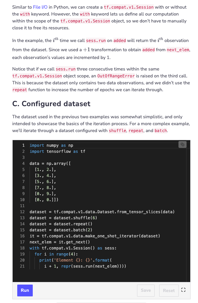
• The first thing to notice is that, despite dataset having only six data observations, we were able to iterate through eight observations because we used the repeat function. In fact, since we used repeat with its default argument setting, we could continuously iterate through the dataset without raising an OutOfRangeError.
• Since we set the batch size to 2 using batch, each iteration returned two data observations rather than 1. Furthermore, you’ll notice that the observations appear in a random order due to shuffle. However, we still saw all the data observations within the first epoch (i.e. first three iterations), because the shuffling occurs on a per-epoch basis.

Feature columns

• Before we get into using a dataset of parsed protocol buffers, we need to first discuss feature columns. In TensorFlow, a feature column is how we specify what kind of data a feature contains. In this chapter, we’ll focus on the two most common types of feature data: numeric and categorical data.
• Feature columns are incredibly useful for converting raw data into an input layer for a machine learning model. Once we have a list of feature columns, we can use them to combine tf.Tensor and tf.SparseTensor feature data into a single input layer. We’ll discuss more of this in the next chapter.
  • B. Numeric features
    • For numeric features, we create a feature column using tf.feature_column.numeric_feature. The function takes in the feature name as a required argument.

import tensorflow as tf

nc = tf.feature_column.numeric_column(
  'GPA', shape=5, dtype=tf.float32)

print(nc)

• In the example above, nc represents a numeric feature column for the feature called ‘GPA’. We used the shape keyword argument to specify that the feature must be 1-D and contain 5 elements. We also set the feature’s datatype to tf.float32.
• Other less commonly used keyword arguments for the function are default_value and normalizer_fn.
• The default_value keyword argument sets the default value for the feature column if the feature is missing from the protocol buffer. If None (which is the default), it means that the specified feature must be present in all entries in order for us to use the numeric column without error.
• The normalizer_fn keyword argument takes in a function that normalizes the feature data. This would be used in a similar way to how map is used for datasets.

Categorical features

• To create a feature column for categorical data, we need a vocabulary for the data. A vocabulary simply refers to the list of possible categories for the data. There are two functions we use to create categorical feature columns:
• tf.feature_column.categorical_column_with_vocabulary_list
• tf.feature_column.categorical_column_with_vocabulary_file
• From this point on, we’ll refer to these functions without their tf.feature_column prefix, for brevity.

import tensorflow as tf

cc1 = tf.feature_column.categorical_column_with_vocabulary_list(
  'name', ['a', 'b', 'c'])

cc2 = tf.feature_column.categorical_column_with_vocabulary_list(
  'name', [1, 2, 3])

cc3 = tf.feature_column.categorical_column_with_vocabulary_list(
  'name', ['a', 'b', 'NA'], default_value=2)

cc4 = tf.feature_column.categorical_column_with_vocabulary_list(
  'name', ['a', 'b', 'c'], num_oov_buckets=2)

• The categorical_column_with_vocabulary_list function takes in two required arguments: the feature name and the list of categories (vocabulary).
• The dtype keyword argument specifies the datatype for the feature column. If dtype is not passed in, the datatype is inferred from the vocabulary list. In our example, cc1 has type tf.string and cc2 has type tf.int32.
• The default_value argument specifies a non-negative default index for an OOV (out-of-vocabulary) category. In our example, each OOV value for cc3 would be mapped to the ‘NA’> category.
• The num_oov_buckets argument specifies the number of OOV “dummy” categories to create. These “dummy” values will be filled when we actually run our TensorFlow computation graph. In our example, we create two “dummy” categories in cc4 for placing OOV values into.
• Note that default_value and num_oov_buckets keyword arguments cannot be used together. default_value assigns an already existing category to catch OOV values, while num_oov_buckets creates new categories to put OOV values in.

import tensorflow as tf

cc1 = tf.feature_column.categorical_column_with_vocabulary_file(
  'name', 'vocab.txt')

cc2 = tf.feature_column.categorical_column_with_vocabulary_file(
  'name', 'vocab.txt', vocabulary_size=4)

Burger
Pizza
Taco
Pasta
Cake
Chicken
Soda
Pie
Rice
Pudding
Muffin

• The categorical_column_with_vocabulary_file function takes in two required arguments: the feature name and the file containing the vocabulary. The vocabulary file must contain a single category per line.
• The vocabulary_size keyword argument specifies how many of the vocabulary categories to use. For cc2, we specified that the feature column only use the first 4 categories of the 11 categories listed in the file. When we don’t set this argument, the function will infer the vocabulary size based on the number of lines in the file.
• The remaining keyword arguments are identical to the ones in categorical_column_with_vocabulary_list.

Indicator wrapping

• Unlike numeric feature columns, categorical feature columns cannot be used directly to create the input layer for a machine learning model. In order to actually use a categorical feature column, we need to convert the categorical data into numeric values. One of the most common ways to do this is with the tf.feature_column.indicator_column function.

import tensorflow as tf

cc = tf.feature_column.categorical_column_with_vocabulary_file(
  'name', 'vocab.txt')

ic = tf.feature_column.indicator_column(cc)
print(ic)

Burger
Pizza
Taco
Pasta
Cake
Chicken
Soda
Pie
Rice
Pudding
Muffin

• The indicator column wrapper converts the categorical data into a count vector. The count vector gives a count of how many times each vocabulary category appears in the feature data. You’ll see an explicit example of count vectors in the next chapter.

Time to Code!

• In this chapter you’ll be completing the create_feature_columns function, which creates a list of feature columns for a variety of features. The feature configurations are given by the input dictionary, config.
• Specifically, you’ll be creating three helper functions: create_list_column, create_file_column, and create_numeric_column. These functions are used to create the necessary feature columns for create_feature_columns:

import tensorflow as tf

def create_feature_columns(config, example_spec, output_features=None):
    if output_features is None:
        output_features = config.keys()
    feature_columns = []
    for feature_name in output_features:
        dtype = example_spec[feature_name].dtype
        feature_config = config[feature_name]
        # HELPER FUNCTIONS USED
        if 'vocab_list' in feature_config:
            feature_col = create_list_column(feature_name, feature_config, dtype)
        elif 'vocab_file' in feature_config:
            feature_col = create_file_column(feature_name, feature_config, dtype)
        else:
            feature_col = create_numeric_column(feature_name, feature_config, dtype)
        feature_columns.append(feature_col)
    return feature_columns

• The create_list_column function creates a categorical feature from a vocabulary list. To do this, we use the tf.feature_column.categorical_column_with_vocabulary_list function.
• Set vocab_feature_col equal to the specified function applied with feature_name and feature_config[‘vocab_list’] as the first two arguments, and dtype=dtype for the keyword argument.
• Since vocab_feature_col is a categorical column, we need to wrap it with an indicator column.
• Set feature_col equal to tf.feature_column.indicator_column applied with vocab_feature_col as the only argument. Then return feature_col.

def create_list_column(feature_name, feature_config, dtype):
    vocab_feature_col = tf.feature_column.categorical_column_with_vocabulary_list(
        feature_name, feature_config['vocab_list'], dtype=dtype)
    feature_col = tf.feature_column.indicator_column(vocab_feature_col)
    return feature_col

Model Execution

• The create_file_column function creates a categorical feature from a vocabulary file. To do this, we use the tf.feature_column.categorical_column_with_vocabulary_file function.
• Set vocab_feature_col equal to the specified function applied with feature_name and feature_config[‘vocab_file’] as the first two arguments, and dtype=dtype for the keyword argument.
• Since vocab_feature_col is a categorical column, we need to wrap it with an indicator column. Set feature_col equal to tf.feature_column.indicator_column applied with vocab_feature_col as the only argument. Then return feature_col.
• The create_numeric_column function creates a numeric feature. To do this, we use the tf.feature_column.numeric_column function.
• Set feature_col equal to the specified function applied with feature_name as the first argument, feature_config[‘shape’] for the shape keyword argument, and dtype for the dtype keyword argument. Then return feature_col.
• In this section you will be learning about the model execution process in TensorFlow. This involves model training, evaluation, and making predictions. The techniques and APIs introduced in the upcoming chapters are used by top industry professionals to easily create organized and efficient machine learning models.
• The first model you create is going to be a classification model. Classification models take data observations and label them with a certain category. For example, classification models can used for tasks like fraud detection, where something is categorized as either fraud or legitimate.
• The second model you create is going to be a regression model. Regression models take data observations and output a number. which which can be used for predicting sales with this course’s supermarket dataset.

Creating a model

• Machine learning models all follow the same format; they require an input layer, apply some computations, and produce an output. In the following chapters, we will cover this entire process using a generic multilayer perceptron (MLP) neural network.
• Development process
  • The development process for a machine learning model involves continuous training and evaluation. Many machine learning models take an incredibly long time to train. Some take days, or even weeks, to finish training.
• Because of this long training time, it is useful to periodically save the current model state while training. This allows us to stop training if we need to and resume training from the same spot at a later date. It also lets us restore previous versions of a trained model, in case something goes wrong or we overtrain.
• Being able to save and restore models in a streamlined fashion is one of TensorFlow’s best features. Another strength of the TensorFlow library is the ability to easily log certain values, such as a model’s accuracy or loss. This is important in making sure we notice any strange occurrences during training.

Training visualizations

• When training a complex neural network, it is useful to have visualizations of the compuation graph and important values to make sure everything is correct. In TensorFlow, there is a tool known as TensorBoard, which lets us visualize all the important aspects of a model.

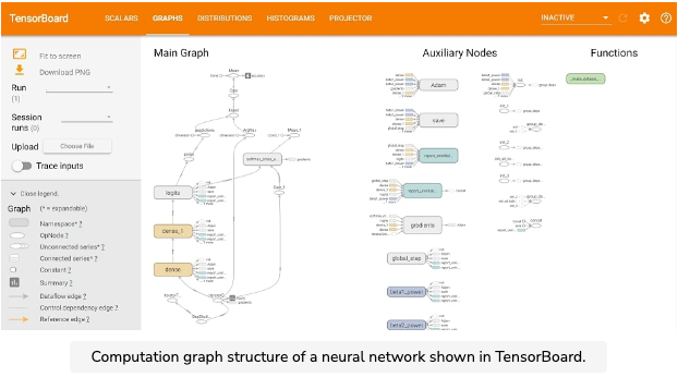
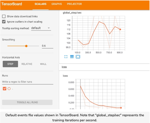
• TensorBoard works by reading in an events file, which contains all the model data we want visualized. When training a model, the events file is stored in the same directory as the model checkpoint (which we’ll discuss in the next chapter). The events file automatically contains the computation graph structure, as well as the loss and training speed (in iterations per second).

• You can run TensorBoard from the command line with the built-in tensorboard module (which comes as part of the TensorFlow library). You just need to specify the directory containing the events file. TensorBoard will then be running in the browser at http://localhost:6006.

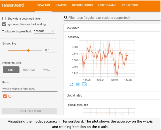
Tracking values

• Apart from the default events file values, we can also specify custom values to track in TensorBoard. To do this, we just need to call tf.summary.scalar in our code.
• The function takes in two required arguments. The first argument is the label name for the visualization in TensorFlow. The second argument is the scalar (i.e. single numeric value) tensor that will be visualized. The tensor’s values will be plotted with respect to the training iterations.

• We can also visualize the distribution of the values for a particular layer in the model. For example, we can view the distribution of the data in the input layer, or we can view the distribution of the weights in a particular hidden layer.
• The function we use to visualize a distribution is tf.summary.histogram. This function takes in the same arguments as tf.summary.scalar.

Time to Code!

• The first seven chapters of this section of the course deals with creating a classification model in TensorFlow, represented by the ClassificationModel object. The function that you’ll be working on this chapter and the next is run_model_training. This function will run training for a classification MLP model and log results to TensorBoard.
• The function calls two helpers:
• dataset_from_numpy: creates a dataset from NumPy data
• run_model_setup: sets up the MLP model Both functions are shown below.

import numpy as np
import tensorflow as tf

class ClassificationModel(object):
    def __init__(self, output_size):
        self.output_size = output_size
 # See the "Efficient Data Processing Techniques" section for details
    def dataset_from_numpy(self, input_data, batch_size, labels=None, is_training=True, num_epochs=None):
        dataset_input = input_data if labels is None else (input_data, labels)
        dataset = tf.compat.v1.data.Dataset.from_tensor_slices(dataset_input)
        if is_training:
            dataset = dataset.shuffle(len(input_data)).repeat(num_epochs)
        return dataset.batch(batch_size)
    
    # See the "Machine Learning for Software Engineers" course on Educative
    def run_model_setup(self, inputs, labels, hidden_layers, is_training, calculate_accuracy=True):
        layer = inputs
        
        for num_nodes in hidden_layers:
            input = tf.keras.Input(tensor = layer)
            layer = tf.keras.layers.Dense( num_nodes,
                activation='relu')(input)
        input_layer = tf.keras.Input(tensor = layer)
        logits = tf.keras.layers.Dense( self.output_size,
            name='logits')(input_layer)
        self.probs = tf.compat.v1.math.softmax(logits, name='probs')
        self.predictions = tf.argmax(
            self.probs, axis=-1, name='predictions')
        if calculate_accuracy:
            class_labels = tf.argmax(labels, axis=-1)
            is_correct = tf.equal(
                self.predictions, class_labels)
            is_correct_float = tf.cast(
                is_correct,
                tf.float32)
            self.accuracy = tf.reduce_mean(
                is_correct_float)
        if labels is not None:
            labels_float = tf.cast(
                labels, tf.float32)
            cross_entropy = tf.compat.v1.nn.softmax_cross_entropy_with_logits_v2(
                labels=labels_float,
                logits=logits)
            self.loss = tf.reduce_mean(
                cross_entropy)
        if is_training:
            adam = tf.compat.v1.train.AdamOptimizer()
            self.train_op = adam.minimize(
                self.loss, global_step=self.global_step)

• In this chapter, you’ll be creating another helper function called add_to_tensorboard, which adds metrics to log in TensorBoardg.
• It’s useful to keep track of how the model accuracy changes while training. Therefore, we’ll want to make sure it’s plotted in TensorBoard.
• Call tf.summary.scalar with ‘accuracy’ as the first argument and self.accuracy as the second argument.
• We also want to store the distribution of the input layer (represented by inputs) in our TensorBoard. To visualize the distribution, we’ll make sure to store it as a histogram.
• Call tf.summary.histogram with ‘inputs’ as the first argument and inputs as the second argument.

class ClassificationModel(object):
    def __init__(self, output_size):
        self.output_size = output_size
    
    # Adds metrics to TensorBoard
    def add_to_tensorboard(self, inputs):
        #CODE HERE
        pass

    # See the "Efficient Data Processing Techniques" section for details
    def dataset_from_numpy(self, input_data, batch_size, labels=None, is_training=True, num_epochs=None):
        dataset_input = input_data if labels is None else (input_data, labels)
        dataset = tf.compat.v1.data.Dataset.from_tensor_slices(dataset_input)
        if is_training:
            dataset = dataset.shuffle(len(input_data)).repeat(num_epochs)
        return dataset.batch(batch_size)
    
    # See the "Machine Learning for Software Engineers" course on Educative
    def run_model_setup(self, inputs, labels, hidden_layers, is_training, calculate_accuracy=True):
        layer = inputs
        
        for num_nodes in hidden_layers:
            input = tf.keras.Input(tensor = layer)
            layer = tf.keras.layers.Dense( num_nodes,
                activation='relu')(input)
        input_layer = tf.keras.Input(tensor = layer)
        logits = tf.keras.layers.Dense( self.output_size,
            name='logits')(input_layer)
        self.probs = tf.compat.v1.math.softmax(logits, name='probs')
        self.predictions = tf.argmax(
            self.probs, axis=-1, name='predictions')
        if calculate_accuracy:
            class_labels = tf.argmax(labels, axis=-1)
            is_correct = tf.equal(
                self.predictions, class_labels)
            is_correct_float = tf.cast(
                is_correct,
                tf.float32)
            self.accuracy = tf.reduce_mean(
                is_correct_float)
        if labels is not None:
            labels_float = tf.cast(
                labels, tf.float32)
            cross_entropy = tf.compat.v1.nn.softmax_cross_entropy_with_logits_v2(
                labels=labels_float,
                logits=logits)
            self.loss = tf.reduce_mean(
                cross_entropy)
        if is_training:
            adam = tf.compat.v1.train.AdamOptimizer()
            self.train_op = adam.minimize(
                self.loss, global_step=self.global_step)
    
    # Run training of the classification model
    def run_model_training(self, input_data, labels, hidden_layers, batch_size, num_epochs, ckpt_dir):
        
        self.global_step = tf.compat.v1.train.get_or_create_global_step()
        dataset = self.dataset_from_numpy(input_data, batch_size,
            labels=labels, num_epochs=num_epochs)
        iterator = tf.compat.v1.data.make_one_shot_iterator(dataset)
        inputs, labels = iterator.get_next()
        self.run_model_setup(inputs, labels, hidden_layers, True)
        self.add_to_tensorboard(inputs)

Logging values

• While tf.summary.scalar lets us keep track of certain values in an events file for TensorBoard, it is also useful to directly log values to STDOUT during training. For instance, it is customary to log the loss and iteration count, so we can stop training if there is an issue.

python train_model.py

• You’ll notice each line of output is prepended by “INFO:tensorflow”. This just means the logging level is set to INFO.
• We log specific values while training using a tf.compat.v1.train.LoggingTensorHook object. The object is initialized with a dictionary mapping labels to scalar valued tensors. In our example, the labels we used were ‘loss’ and ‘step’, for the loss and iteration count tensors, respectively. In the run_model_training function, self.loss represents the loss tensor and self.global_step represents the iteration count, also known as the training step.
• To specify the logging frequency, we need to set exactly one of every_n_iter or every_n_secs as a keyword argument when initializing tf.compat.v1.train.LoggingTensorHook. In the example above, we set every_n_iter to 100, so that logging is shown every 100 iterations.
• We can also use every_n_secs to specify a time interval for displaying logged values.

Catching NaN

• In addition to logging values during training, we also want to automatically stop training if the loss ever takes on an infinite value. In TensorFlow, similar to NumPy, an infinite value is represented by NaN.

python3 train_model_nan.py

• We use the tf.compat.v1.train.NanTensorHook to handle NaN loss. When initializing tf.compat.v1.train.NanTensorHook, we only need to pass in the loss tensor variable as a required argument.

Efficient training

• We can use tf.compat.v1.Session and tf.compat.v1.placeholder to run model training. However, this is a relatively inefficient training method, and should really only be used to train small models or run tests/evaluation.
• We’ve already shown how to replace tf.compat.v1.placeholder for the input data, by iterating through a TensorFlow dataset. We can also replace tf.compat.v1.Session with tf.compat.v1.train.MonitoredTrainingSession, which handles a lot of the training dirty work for us.
• The >MonitoredTrainingSession will initialize all the necessary variables in the computation graph and log specified scalar values. We can run training within the scope of a MonitoredTrainingSession object by using the with keyword.
• Below we show how to use a MonitoredTrainingSession object.

log_vals = {
    'loss': model_loss,
    'step': global_step
}
log_hook = tf.compat.v1.train.LoggingTensorHook(log_vals, every_n_iter=10)
nan_hook = tf.compat.v1.train.NanTensorHook(model_loss)
hooks = [nan_hook, log_hook]
with tf.compat.v1.train.MonitoredTrainingSession(
    hooks=hooks) as sess:
    while not sess.should_stop():
        sess.run(train_op)

• In the example above, we specified that the training will log the loss and training step every 10 iterations, as well as handle NaN loss. Note that we pass in the logging and NaN hooks as a list with the hooks keyword argument.
• The should_stop function returns a boolean value representing whether the training should stop. It will return true if it reaches the end of the dataset, catches an error (e.g. Nan loss), or a kill signal is sent from the keyboard with CTRL+C or CMD+C. Using should_stop in a while loop will check whether we continue training after each iteration.

Checkpoints

• One of the most important utilities provided by MonitoredTrainingSession is the ability to create a checkpoint directory. A checkpoint refers to a saved model state after a specific training iteration. We can save multiple checkpoints and store them in the checkpoint directory, which will also contain the events file used for TensorBoard.
• Below we show how to use a MonitoredTrainingSession to save the model state as a checkpoint.

log_vals = {
    'loss': model_loss,
    'step': global_step
}
log_hook = tf.compat.v1.train.LoggingTensorHook(log_vals, every_n_iter=10)
nan_hook = tf.compat.v1.train.NanTensorHook(model_loss)
hooks = [nan_hook, log_hook]
ckpt_dir = 'my_model'
with tf.compat.v1.train.MonitoredTrainingSession(
    checkpoint_dir=ckpt_dir,
    hooks=hooks) as sess:
    while not sess.should_stop():
        sess.run(train_op)

• In the example above, we saved the model checkpoints in the my_model directory, by setting the checkpoint_dir keyword argument accordingly. Notice that when we specify a checkpoint directory, the global_step/sec metric is also logged, since it is tracked by default in TensorBoard.
• If we run training again using the same checkpoint directory, it will restore the model state from the most recent checkpoint. This is extremely helpful since it allows us to stop and start training at different times, without losing any progress.

Model code

• In the ClassificationModel, we use the MonitoredTrainingSession object to run training and save the model state to a checkpoint. The finished run_model_training code is shown below:

def run_model_training(self, input_data, labels, hidden_layers, batch_size, num_epochs, ckpt_dir):
    self.global_step = tf.compat.v1.train.get_or_create_global_step()
    dataset = self.dataset_from_numpy(input_data, batch_size,
        labels=labels, num_epochs=num_epochs)
    iterator = tf.compat.v1.data.make_one_shot_iterator(dataset)
    inputs, labels = iterator.get_next()
    self.run_model_setup(inputs, labels, hidden_layers, True)
    self.add_to_tensorboard(inputs)
    log_vals = {'loss': self.loss, 'step': self.global_step}
    logging_hook = tf.compat.v1.train.LoggingTensorHook(
        log_vals, every_n_iter=1000)
    nan_hook = tf.compat.v1.train.NanTensorHook(self.loss)
    hooks = [nan_hook, logging_hook]
    with tf.compat.v1.train.MonitoredTrainingSession(
        checkpoint_dir=ckpt_dir,
        hooks=hooks) as sess:
        while not sess.should_stop():
            sess.run(self.train_op)

Checkpoint directory

• After running training with a checkpoint directory, it will contain several files. An example checkpoint directory, named my_model, is shown below.

ls my_model

• The .pbtxt file represents the entire computation graph stored in human readable text format. The .tfevents file is the events file for TensorBoard (note that the longer file suffix, which contains the local machine’s ID, is omitted).
• The actual saved model state at a particular training step consists of the following three files:
  • data: One or more files containing the values for the model’s parameters. Larger models may require more .data files.
  • .index: Metadata descriptions for how to find a particular tensor in the .data file(s).
  • .meta: Represents the non-human readable saved graph structure. This file can be used to restore the computation graph.
• The checkpoint file lists which checkpoint to use when restoring parameters, as well as all the possible checkpoints available.

cat my_model/checkpoint

Saving parameters

• The traditional method to save and restore parameters in TensorFlow is to use the tf.compat.v1.train.Saver object.
• To save the parameters of a given TensorFlow session, use tf.compat.v1.train.Saver.save. This function has two required arguments: the current session and the path to which the file will be saved.
• It has many keyword arguments, one of which is global_step, which determines the number tacked on to the back of the file name.

# sess is a tf.Session object
# 'my-model' is the filepath
# global_step 
saver.save(sess, 'my-model', global_step=1000)
# checkpoint filename will be 'my-model-1000'
# the file will be in the current working directory

Restoring parameters

• When we use MonitoredTrainingSession to resume training, it automatically restores parameters from the model_checkpoint_path specified in the checkpoint file. However, if we want to evaluate the model or use it for predictions, we need another way to restore the parameters.
• The tf.compat.v1.train.Saver.restore function is the way to do that.

import tensorflow as tf
inputs = tf.keras.Input(inputs)
logits = tf.keras.layers.Dense(1)(inputs)

saver = tf.compat.v1.train.Saver()
ckpt = tf.compat.v1.train.get_checkpoint_state('my_model')
if ckpt is not None:  # Check if has checkpoint file
  sess = tf.compat.v1.Session()
  saver.restore(sess, ckpt.model_checkpoint_path)
  sess.run(logits)

• In the example above, we obtain the checkpoint state of my_model with the tf.compat.v1.train.get_checkpoint_state function. The function returns a CheckpointState object which contains the properties model_checkpoint_path and all_checkpoint_paths. The former represents the checkpoint to use, while the latter represents the list of all checkpoints. Note that if the checkpoint file is not present in the checkpoint directory, the function returns None.
• The Saver object contains the restore function, which restores the checkpoint from the path given in the second argument. The first argument is a tf.compat.v1.Session object that we use to execute the restoration.
• We can use the save function to save the computation graph’s parameters. It takes in the same two required arguments as restore, and saves the parameters to the directory passed in as the second argument.

Training vs. evaluation

• To measure how well our model has been trained, we evaluate it on datasets other than the training set. The datasets used for evaluation are known as the validation and test sets. Note that we don’t shuffle or repeat the evaluation datasets, since those are techniques used specifically to improve training.
• The validation set is used to evaluate a model in between training runs. We use the validation set to tweak certain hyperparameters for a model (such as learning rate or batch size) in order to make sure training continues smoothly. We also use the validation set to detect model overfitting, so we can stop training if overfitting is detected.

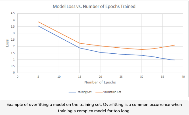
• Overfitting occurs when we train a model (usually a relatively complex model) for too long on the training set, resulting in a decreased ability to generalize well to other datasets. In the above plot, overfitting occurs around the 32nd epoch of training, when the loss on the validation set begins to increase.
• The test set is used to evaluate the final version of a model, after it is completely done training. Evaluating on the test set lets us know how well our model performs on its given task.

Evaluation metrics

• There are a variety of different metrics that can be used for evaluation, depending on the application that a model is built for. However, a universal evaluation metric for machine learning models is the loss. Since every machine learning model is trained to minimize some loss metric, it is natural to use that loss metric during evaluation.
• Another commonly used evaluation metric for classification models is accuracy. This refers to the fraction of dataset observations that a machine learning model can label with the correct class. While we train a classification model by minimizing the loss (normally cross entropy), the true goal is to increase model accuracy when classifying new data.

Time to Code!

• In this chapter you’ll be completing the evaluate_saved_model function, which restores a classification model from a checkpoint and then runs evaluation on the model.
• First, we get the checkpoint state from the checkpoint directory and make sure the checkpoint file is there.
• Set ckpt equal to tf.compat.v1.train.get_checkpoint_state applied with ckpt_dir as the only argument.
• Then create an if block that checks if ckpt is not None.
• If the checkpoint state is correct, we can set up a Saver object and restore the model parameters.
• Inside the if block, set saver equal to a tf.compat.v1.train.Saver object, initialized with no arguments.
• Then call saver.restore with sess and ckpt.model_checkpoint_path as the two input arguments.
• The evaluation metrics we return are the model accuracy and loss. We’ll use the input argument sess (a tf.compat.v1.Session object) to extract the metrics.
• Inside the if block, set eval_metrics equal to sess.run with the tuple (self.accuracy, self.loss) as the only argument.
• Then return eval_metrics.

import numpy as np
import tensorflow as tf

class ClassificationModel(object):
    def __init__(self, output_size):
        self.output_size = output_size
    
    # Run model evaluation
    def evaluate_saved_model(self, sess, ckpt_dir):
        # CODE HERE
        pass

    # See the "Efficient Data Processing Techniques" section for details
    def dataset_from_numpy(self, input_data, batch_size, labels=None, is_training=True, num_epochs=None):
        dataset_input = input_data if labels is None else (input_data, labels)
        dataset = tf.data.Dataset.from_tensor_slices(dataset_input)
        if is_training:
            dataset = dataset.shuffle(len(input_data)).repeat(num_epochs)
        return dataset.batch(batch_size)
    
    # See the "Machine Learning for Software Engineers" course on Educative
    def run_model_setup(self, inputs, labels, hidden_layers, is_training, calculate_accuracy=True):
        layer = inputs
        
        for num_nodes in hidden_layers:
            input = tf.keras.Input(tensor = layer)
            layer = tf.keras.layers.Dense( num_nodes,
                activation='relu')(input)
        input_layer = tf.keras.Input(tensor = layer)
        logits = tf.keras.layers.Dense( self.output_size,
            name='logits')(input_layer)
        self.probs = tf.compat.v1.math.softmax(logits, name='probs')
        self.predictions = tf.math.argmax(
            self.probs, axis=-1, name='predictions')
        if calculate_accuracy:
            class_labels = tf.math.argmax(labels, axis=-1)
            is_correct = tf.equal(
                self.predictions, class_labels)
            is_correct_float = tf.cast(
                is_correct,
                tf.float32)
            self.accuracy = tf.math.reduce_mean(
                is_correct_float)
        if labels is not None:
            labels_float = tf.cast(
                labels, tf.float32)
            cross_entropy = tf.compat.v1.nn.softmax_cross_entropy_with_logits_v2(
                labels=labels_float,
                logits=logits)
            self.loss = tf.reduce_mean(
                cross_entropy)
        if is_training:
            adam = tf.compat.v1.train.AdamOptimizer()
            self.train_op = adam.minimize(
                self.loss, global_step=self.global_step)
    
    # Run training of the classification model
    def run_model_training(self, input_data, labels, hidden_layers, batch_size, num_epochs, ckpt_dir):
        self.global_step = tf.compat.v1.train.get_or_create_global_step()
        dataset = self.dataset_from_numpy(input_data, batch_size,
            labels=labels, num_epochs=num_epochs)
        iterator = tf.compat.v1.data.make_one_shot_iterator(dataset)
        inputs, labels = iterator.get_next()
        self.run_model_setup(inputs, labels, hidden_layers, True)
        tf.summary.scalar('accuracy', self.accuracy)
        tf.summary.histogram('inputs', inputs)
        log_vals = {'loss': self.loss, 'step': self.global_step}
        logging_hook = tf.compat.v1.train.LoggingTensorHook(
            log_vals, every_n_iter=1000)
        nan_hook = tf.compat.v1.train.NanTensorHook(self.loss)
        hooks = [nan_hook, logging_hook]
        with tf.compat.v1.train.MonitoredTrainingSession(
            checkpoint_dir=ckpt_dir,
            hooks=hooks) as sess:
            while not sess.should_stop():
                sess.run(self.train_op)

Save For Inference

Deploying a model

• As mentioned in chapter 4, a saved model checkpoint consists of three files: .data, .index, and .meta. Since the .meta file contains the entire computation graph structure, which includes all the data in the training dataset, it can get quite large. The large file size becomes an issue when deploying an inference model.
• An inference model is a fully trained and evaluated model used to make predictions on real-time data. When we deploy an inference model for production, we don’t usually deploy the code used to build the model, either for proprietary reasons or because there are too many auxiliary code files. When we don’t have the code that sets up the inference graph, we need a separate file that specifies the computation graph’s structure.

Inference graph

• The main issue with the .meta file is that it contains many unnecessary portions of the computation graph, with respect to inference. For inference, we only need a tf.compat.v1.placeholder to represent the input data. We also don’t need any parts of the computation graph specific to training, such as the loss calculation or dataset.
• So instead of using a training checkpoint for the inference model, we create a bare-bones computation graph, consisting only of the input placeholder and the computations necessary to obtain a prediction.
• If the model just finished training (meaning the training computation graph is still in memory), it’s necessary to use tf.compat.v1.reset_default_graph prior to building the inference graph, in order to avoid graph conflicts.

import tensorflow as tf

inputs = tf.compat.v1.placeholder(
    tf.float32, shape=(None, 3), name='inputs')
logits = tf.keras.layers.Dense( 1, name='logits')(inputs)
try:
    logits = tf.keras.layers.Dense(1, name='logits')(inputs)
except ValueError: # Need to reset graph
    tf.inputs,reset_default_graph()
    inputs = tf.compat.v1.placeholder(
        tf.float32, shape=(None, 3), name='inputs')
    logits = tf.keras.layers.Dense( 1, name='logits')(inputs)
    print(logits)

Saving the model

• We save the inference model using tf.compat.v1.saved_model.simple_save. The function’s first argument is a tf.compat.v1.Session object and the second argument is the path to the directory where we save the inference model. Note that the directory with which we save the inference model must not already exist.
• The third argument is a dictionary containing the input tensor(s) as values, with string labels as keys. The fourth required argument is also a dictionary with string keys, but for the output tensor(s), e.g. the model prediction.
• The function will save a file called saved_model.pb and a directory called variables in the specified directory.

ls inference_dir

• In the example above, inference_dir is the directory where tf.compat.v1.saved_model.simple_save saved the inference model. The saved_model.pb file contains the bare-bones computation graph, and is much smaller than the corresponding .meta file. The variables directory contains the model’s saved parameters.
• In the next chapter, you’ll learn how to restore the inference model and make predictions.

Time to Code!

• In this chapter you’ll complete the save_inference_graph function, which saves the model’s computation graph for inference. The function is already filled with code that restores the model state from a checkpoint.
• The input dictionary for the inference graph contains input_placeholder as its only value, which represents the input data for the inference graph.
• Set input_dict equal to a dictionary with a single key, ‘inputs’, that maps to input_placeholder.
• The output dictionary for the inference graph contains self.predictions as its only value. The corresponding key is ‘predictions’.
• Set output_dict equal to a dictionary consisting of the specified key-value pair.
• After creating the dictionaries for the inference graph’s input and output, we can save the model using tf.compat.v1.saved_model.simple_save.
• Call the specified function with sess, export_dir, input_dict, and output_dict as the four input arguments.

import numpy as np
import tensorflow as tf

class ClassificationModel(object):
    def __init__(self, output_size):
        self.output_size = output_size
    
    # Save the model's computation graph for inference
    def save_inference_graph(self, sess, ckpt_dir, input_placeholder, export_dir):
        ckpt = tf.compat.v1.train.get_checkpoint_state(ckpt_dir)
        if ckpt is not None:
            saver = tf.compat.v1.train.Saver()
            saver.restore(sess, ckpt.model_checkpoint_path)
            #CODE HERE
            pass

    # See the "Efficient Data Processing Techniques" section for details
    def dataset_from_numpy(self, input_data, batch_size, labels=None, is_training=True, num_epochs=None):
        dataset_input = input_data if labels is None else (input_data, labels)
        dataset = tf.compat.v1.data.Dataset.from_tensor_slices(dataset_input)
        if is_training:
            dataset = dataset.shuffle(len(input_data)).repeat(num_epochs)
        return dataset.batch(batch_size)
    
    # See the "Machine Learning for Software Engineers" course on Educative
    def run_model_setup(self, inputs, labels, hidden_layers, is_training, calculate_accuracy=True):
        layer = inputs
        for num_nodes in hidden_layers:
            layer = tf.keras.layers.Dense( num_nodes,
                activation=tf.nn.relu)(layer)
        logits = tf.keras.layers.Dense( self.output_size,
            name='logits')(layer)
        self.probs = tf.compat.v1.nn.softmax(logits, name='probs')
        self.predictions = tf.math.argmax(
            self.probs, axis=-1, name='predictions')
        if calculate_accuracy:
            class_labels = tf.math.argmax(labels, axis=-1)
            is_correct = tf.equal(
                self.predictions, class_labels)
            is_correct_float = tf.cast(
                is_correct,
                tf.float32)
            self.accuracy = tf.math.reduce_mean(
                is_correct_float)
        if labels is not None:
            labels_float = tf.cast(
                labels, tf.float32)
            cross_entropy = tf.compat.v1.nn.softmax_cross_entropy_with_logits_v2(
                labels=labels_float,
                logits=logits)
            self.loss = tf.math.reduce_mean(
                cross_entropy)
        if is_training:
            adam = tf.compat.v1.train.AdamOptimizer()
            self.train_op = adam.minimize(
                self.loss, global_step=self.global_step)
    
    # Run training of the classification model
    def run_model_training(self, input_data, labels, hidden_layers, batch_size, num_epochs, ckpt_dir):
        self.global_step = tf.compat.v1.train.get_or_create_global_step()
        dataset = self.dataset_from_numpy(input_data, batch_size,
            labels=labels, num_epochs=num_epochs)
        iterator = tf.compat.v1.data.make_one_shot_iterator(dataset)
        inputs, labels = iterator.get_next()
        self.run_model_setup(inputs, labels, hidden_layers, True)
        tf.summary.scalar('accuracy', self.accuracy)
        tf.summary.histogram('inputs', inputs)
        log_vals = {'loss': self.loss, 'step': self.global_step}
        logging_hook = tf.compat.v1.train.LoggingTensorHook(
            log_vals, every_n_iter=1000)
        nan_hook = tf.compat.v1.train.NanTensorHook(self.loss)
        hooks = [nan_hook, logging_hook]
        with tf.compat.v1.train.MonitoredTrainingSession(
            checkpoint_dir=ckpt_dir,
            hooks=hooks) as sess:
            while not sess.should_stop():
                sess.run(self.train_op)

Predictions

• Restore an inference model and make predictions on an input dataset.

Restoring the model

• To restore an inference model, we use the tf.compat.v1.saved_model.loader.load function. This function restores both the inference graph as well as the inference model’s parameters.
• Since the function’s first argument is a tf.compat.v1.Session object, it’s a good idea to restore the inference model within the scope of a particular tf.compat.v1.Session.

import tensorflow as tf

tags = [tf.compat.v1.saved_model.tag_constants.SERVING]
model_dir = 'inference_model'
with tf.compat.v1.Session(graph=tf.Graph()) as sess:
    tf.saved_model.loader.load(sess, tags, model_dir)

• The second argument for tf.compat.v1.saved_model.loader.load is a list of tag constants. For inference, we use the SERVING tag. The function’s third argument is the path to the saved inference model’s directory.
• In the example above, we restored the inference model within the scope of a tf.compat.v1.Session object named sess. Note that sess is initialized with a new, empty computation graph in tf.Graph(). This ensures that there are no graph conflicts, similar to tf.compat.v1.reset_default_graph, but also that it doesn’t erase the graph outside the scope of sess.

Retrieving tensors

• After restoring the inference model, the inference graph is represented by sess.graph, which is a Graph object. We use the Graph object’s get_tensor_by_name function to retrieve specific tensors from the computation graph.

import tensorflow as tf

tags = [tf.compat.v1.saved_model.tag_constants.SERVING]
model_dir = 'inference_model'
with tf.compat.v1.Session(graph=tf.Graph()) as sess:
    tf.compat.v1.saved_model.loader.load(sess, tags, model_dir)
    preds = sess.graph.get_tensor_by_name('predictions:0')

• The input argument for get_tensor_by_name is the name of the tensor we wish to retrieve. In the above example, the tensor name has :0 as a suffix. Whenever we retrieve a single tensor from the computation graph, we need to add the :0 suffix.

Time to Code!

• In this chapter you’ll be completing the make_predictions function, which makes predictions using a saved inference graph. Specifically, you’ll be creating the helper function load_inference_parts, which loads the inference graph and gets the necessary tensors.
• We can load the saved inference model using the function tf.compat.v1.saved_model.loader.load. The tag list we use to load the inference model is a singleton list containing tf.compat.v1.saved_model.tag_constants.SERVING.
• Call the loading function with sess, the specified tag list, and saved_model_dir as the three input arguments.
• Next, we’ll get the input placeholder and the predictions tensor from the loaded computation graph. The computation graph corresponds to sess.graph, and we use sess.graph.get_tensor_by_name to retrieve a specific tensor based on its name.
• Set inputs equal to the tensor retrieving function with ‘inference_input:0’ as the only argument.
• Set predictions_tensor equal to the tensor retrieving function with ‘predictions:0’ as the only argument.
• Since the model probabilities are used to calculate the predictions, the probabilities tensor is part of the computation graph. Therefore, we can retrieve the tensor using its name.
• Set probs_tensor equal to the tensor retrieving function with ‘probs:0’ as the only argument.
• Return a tuple containing inputs as the first element, predictions_tensor as the second element, and probs_tensor as the third element.

import numpy as np
import tensorflow as tf

class ClassificationModel(object):
    def __init__(self, output_size):
        self.output_size = output_size

    # Helper for make_predictions
    def load_inference_parts(self, sess, saved_model_dir):
        # CODE HERE
        pass
    
    # Make predictions with the inference model
    def make_predictions(self, saved_model_dir, input_data):
        with tf.compat.v1.Session(graph=tf.Graph()) as sess:
            inputs, predictions_tensor, probs_tensor = self.load_inference_parts(sess, saved_model_dir)
            predictions, probs = sess.run((predictions_tensor, probs_tensor), feed_dict={inputs: input_data})
        return predictions, probs

    # See the "Efficient Data Processing Techniques" section for details
    def dataset_from_numpy(self, input_data, batch_size, labels=None, is_training=True, num_epochs=None):
        dataset_input = input_data if labels is None else (input_data, labels)
        dataset = tf.compat.v1.data.Dataset.from_tensor_slices(dataset_input)
        if is_training:
            dataset = dataset.shuffle(len(input_data)).repeat(num_epochs)
        return dataset.batch(batch_size)
    
    # See the "Machine Learning for Software Engineers" course on Educative
    def run_model_setup(self, inputs, labels, hidden_layers, is_training, calculate_accuracy=True):
        layer = inputs
        
        for num_nodes in hidden_layers:
            input = tf.keras.Input(tensor = layer)
            layer = tf.keras.layers.Dense( num_nodes,
                activation='relu')(input)
        input_layer = tf.keras.Input(tensor = layer)
        logits = tf.keras.layers.Dense( self.output_size,
            name='logits')(input_layer)
        self.probs = tf.compat.v1.math.softmax(logits, name='probs')
        self.predictions = tf.argmax(
            self.probs, axis=-1, name='predictions')
        if calculate_accuracy:
            class_labels = tf.argmax(labels, axis=-1)
            is_correct = tf.equal(
                self.predictions, class_labels)
            is_correct_float = tf.cast(
                is_correct,
                tf.float32)
            self.accuracy = tf.reduce_mean(
                is_correct_float)
        if labels is not None:
            labels_float = tf.cast(
                labels, tf.float32)
            cross_entropy = tf.compat.v1.nn.softmax_cross_entropy_with_logits_v2(
                labels=labels_float,
                logits=logits)
            self.loss = tf.reduce_mean(
                cross_entropy)
        if is_training:
            adam = tf.compat.v1.train.AdamOptimizer()
            self.train_op = adam.minimize(
                self.loss, global_step=self.global_step)
    
    # Run training of the classification model
    def run_model_training(self, input_data, labels, hidden_layers, batch_size, num_epochs, ckpt_dir):
        self.global_step = tf.train.get_or_create_global_step()
        dataset = self.dataset_from_numpy(input_data, batch_size,
            labels=labels, num_epochs=num_epochs)
        iterator = tf.compat.v1.data.make_one_shot_iterator(dataset)
        inputs, labels = iterator.get_next()
        self.run_model_setup(inputs, labels, hidden_layers, True)
        tf.summary.scalar('accuracy', self.accuracy)
        tf.summary.histogram('inputs', inputs)
        log_vals = {'loss': self.loss, 'step': self.global_step}
        logging_hook = tf.compat.v1.train.LoggingTensorHook(
            log_vals, every_n_iter=1000)
        nan_hook = tf.compat.v1.train.NanTensorHook(self.loss)
        hooks = [nan_hook, logging_hook]
        with tf.compat.v1.train.MonitoredTrainingSession(
            checkpoint_dir=ckpt_dir,
            hooks=hooks) as sess:
            while not sess.should_stop():
                sess.run(self.train_op)
    

• Below is an example plot of some predictions (run the show_plot() function). The points in this plot represent the winning percentages of MLB teams in 2017.
• The plot’s z-axis corresponds to winning percentage, the y-axis corresponds to runs per game, and the x-axis corresponds to batting average.
• The inference model was trained on runs per game and batting average to classify a team into one of three classes:
• Poor: Winning percentage below 0.450 (73 wins)
• Average: Winning percentage between 0.450 and 0.543 (88 wins)
• Good: Winning percentage above 0.543
• The winning percentage thresholds are represented by the two planes in the 3-D plot. Correct predictions by the model are marked in blue, while incorrect predictions are marked in red.
• If you hover over any of the points, it will give you information on the model’s prediction and probability per class

Regression

• Understand the difference between regression and classification models.

Classification vs. regression

• The model we’ve been using so far is built for classification. This means it classifies input data into one of many different classes.
• While classification is one of the most important tasks that can be done by a neural network, another common application of neural networks is regression. Rather than assigning the input data to a particular class, a regression model will instead output a real number value based on the input data. Regression tasks can range from predicting stock prices to predicting the future height of a child.
• Classification models obtain probabilities and class predictions from the calculated logits. A regression model can just return the logits, since the logits represent the real-valued output of the model’s layers.

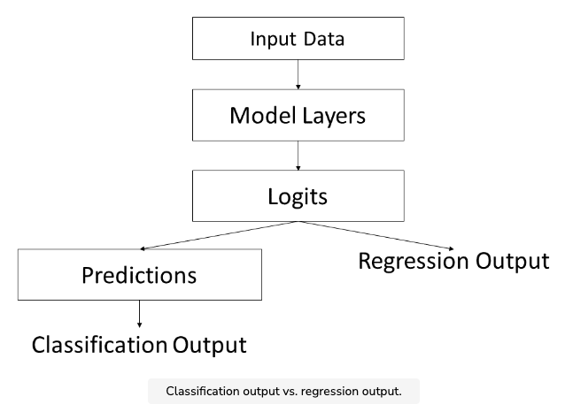
L2 loss

• When training a classification model, the loss function we use is the cross entropy loss. For regression models, we normally use the L2 loss, which is a loss function derived from the L2-norm.
• In TensorFlow, the L2 loss is calculated by the tf.compat.v1.nn.l2_loss function. Note that the TensorFlow implementation omits the square root used in the L2-norm and also divides the value by 2. This makes it easier to calculate the gradient for weight optimization.
• We normally use L2 loss on the subtracted difference between two scalars or tensors. The L2 loss represents how “close” the two values are.

import tensorflow as tf
t1 = tf.constant([9.3, 95.4, -0.3])
t2 = tf.constant([9.35, 95.4, -0.28])
t3 = tf.constant([-80.4, -95.1, 78])
with tf.compat.v1.Session() as sess:
  print(sess.run(tf.compat.v1.nn.l2_loss(t1 - t2)))
  print(sess.run(tf.compat.v1.nn.l2_loss(t1 - t3)))

• An L2 loss near 0 means the two values are very close, while a large L2 loss means the values are not close at all. In our example, the elements of t1 and t2 are extremely close, so their L2 loss is tiny. On the other hand, t1 and t3 are not close at all, so their L2 loss is large.
• For regression models, we calculate the L2 loss between the model’s output (i.e. logits) and the labels for the input data.

Time to Code!

• In this chapter you’ll be completing part of the regressor_fn function, which is the main function for the regression model (RegressionModel) that will be created in this section of the course.
• Specifically, you’ll be completing the helper function set_predictions_and_loss`, which sets the regression predictions and loss (if necessary).
• The logits input argument, which represents the regression model’s logits, has shape (batch_size, 1). However, we want our model predictions to have the same shape as labels, which is `(batch_size,).
• In this case, we use tf.compat.v1.squeeze to remove the size 1 second dimension from logits. The new 1-D tensor corresponds to our model predictions.
• Set self.predictions equal to tf.compat.v1.squeeze with logits as the only argument.
• If labels is specified, we want to compute the regression loss. The loss function used for regression is tf.compat.v1.nn.l2_loss.
• If labels is not None, set self.loss equal to tf.compat.v1.nn.l2_loss applied to the difference between labels and self.predictions.

import numpy as np
import tensorflow as tf

class RegressionModel(object):
    def __init__(self, output_size):
        self.output_size = output_size

    # Helper for regressor_fn
    def set_predictions_and_loss(self, logits, labels):
        # CODE HERE
        
    
    # The function for the regression model
    def regressor_fn(self, features, labels, mode, params):
        inputs = tf.compat.v1.feature_column.input_layer(features, params['feature_columns'])
        layer = inputs
        for num_nodes in params['hidden_layers']:
            input_ = tf.keras.Input(tensor = layer)
            layer = tf.keras.layers.Dense( num_nodes,
                activation='relu')(input_)
        input_layer = tf.keras.Input(tensor = layer)
        logits = tf.keras.layers.Dense( self.output_size,
            name='logits')(input_layer)
        self.set_predictions_and_loss(logits, labels)
        if mode == tf.compat.v1.estimator.ModeKeys.TRAIN:
            self.global_step = tf.compat.v1.train.get_or_create_global_step()
            adam = tf.compat.v1.train.AdamOptimizer()
            self.train_op = adam.minimize(
                self.loss, global_step=self.global_step)
        if mode == tf.compat.v1.estimator.ModeKeys.EVAL:
            pass
        if mode == tf.compat.v1.estimator.ModeKeys.PREDICT:
            pass