Primers • Distributed Systems Handbook
- Overview
- What a distributed system is
- Why distributed systems exist
- The core problem: useful coordination without perfect knowledge
- The basic tradeoffs
- A small set of equations that appear repeatedly
- The implementation lens
- The main conceptual layers
- Distributed systems as control loops
- What “advanced” means in deployed systems
- Primer roadmap
- Foundations
- System model
- Safety and liveness
- Failure models
- Network assumptions and the fallacies of distributed computing
- Time, clocks, and causality
- Lamport clocks
- Vector clocks
- Physical clocks, leases, and clock skew
- Global state and distributed snapshots
- Consensus and the FLP boundary
- CAP and PACELC
- Consistency vocabulary at the foundation layer
- Idempotency, retries, and duplicate-safe design
- Monotonicity and version checks
- Membership and epochs
- Backpressure and bounded queues
- Partial failure as the default
- What every production design should specify
- Communication
- Why communication is the first practical distributed-systems problem
- The communication spectrum
- Synchronous RPC
- Remote-call outcome states
- Retries, backoff, jitter, and retry budgets
- Hedging
- Asynchronous messaging
- Delivery semantics
- Durable logs and streams
- Offset management
- Ordering
- Schema evolution
- Inbox pattern
- Backpressure and flow control
- Load shedding and overload control
- Fanout and tail latency
- Circuit breakers
- Request context propagation
- Serialization and protocol choices
- Gossip and epidemic communication
- Watch APIs and reconciliation
- Communication anti-patterns
- Deployment checklist for communication
- Replication and Consensus
- Why replication exists
- Replicated state machines
- Quorum replication
- Flexible quorums
- Chain replication
- Primary-backup replication
- Consensus as ordered agreement
- Paxos
- Multi-Paxos
- Raft
- Raft leader election
- Raft log replication
- Why terms and epochs matter
- Read paths in consensus systems
- Snapshots and log compaction
- Membership and reconfiguration
- Viewstamped Replication and Zab
- Coordination services
- Leader election with a coordination service
- Split brain
- Geo-replication and consensus placement
- Replication lag
- Anti-entropy and repair
- Replication and external side effects
- Consensus performance knobs
- Consensus availability
- Consensus and deployment systems
- Implementation checklist for a consensus-backed service
- Common replication and consensus failure modes
- Design guidance
- Consistency Models
- Why consistency models matter
- Histories, operations, and legal executions
- The two axes: object consistency and transactional isolation
- A hierarchy of common consistency models
- Linearizability
- Strict serializability
- Serializability
- Sequential consistency
- Causal consistency
- Eventual consistency
- Quorum consistency and tunable reads
- Bounded staleness
- Snapshot isolation
- Read committed, repeatable read, and serializable in practice
- Consistency and constraints
- Choosing consistency per operation
- Testing consistency
- Implementation patterns by model
- Common consistency failure modes
- Deployment checklist for consistency
- Data Partitioning and Sharding
- All writes for the day hit one logical partition key.
- Preserves order for one order.
- Preserves order for one customer, but may hotspot large customers.
- Partitioning in application-sharded databases
- Resharding without downtime
- Partition-aware observability
- Query planning over partitions
- Partitioning and caches
- Design checklist for partitioning
- Common partitioning failure modes
- Distributed Storage
- Why distributed storage is different from local storage
- Storage abstractions
- The storage stack
- Write-ahead logging
- fsync, group commit, and durability latency
- Checksums and corruption detection
- Local storage engines: B-trees and LSM trees
- Memtables, SSTables, and Bloom filters
- Compaction
- Tombstones and deletes
- Distributed filesystems: GFS and HDFS
- Object storage: S3-style systems
- Object placement and CRUSH
- Replication versus erasure coding
- Metadata is often the real bottleneck
- Wide-column storage: Bigtable-style design
- Dynamo-style storage
- Distributed SQL storage
- Snapshots
- Backup and restore
- Garbage collection
- Repair, anti-entropy, and scrubbing
- Read repair
- Storage placement and failure domains
- Capacity management
- Tiering and lifecycle management
- Storage consistency contracts
- Change data capture and storage logs
- Multi-region storage
- Storage for Kubernetes and control planes
- Storage for ML and AI systems
- Manifest files and atomic visibility
- Security in distributed storage
- Common distributed storage failure modes
- Deployment checklist for distributed storage
- Transactions and Workflows
- Why transactions and workflows are separate but related
- ACID properties
- Single-partition transactions
- Cross-partition transactions
- Two-phase commit
- 2PC failure states
- 2PC over replicated participants
- Paxos Commit
- Three-phase commit and why it is rare
- Two-phase locking
- Optimistic concurrency control
- MVCC and transaction timestamps
- Write skew and invariant protection
- Escrow and bounded counters
- Compare-and-swap and conditional writes
- Idempotency for transaction boundaries
- The dual-write problem
- Inbox and deduplicated consumers
- Kafka transactions and exactly-once stream processing
- Sagas
- Orchestration versus choreography
- Workflow engines
- Try-confirm-cancel
- Human-in-the-loop workflows
- Workflow state machines
- Durable execution versus distributed transactions
- Exactly-once business effects
- Reconciliation
- Compensating transactions
- Dead-letter queues and poison workflow steps
- Workflow observability
- Transaction and workflow testing
- Concrete design examples
- Choosing the right mechanism
- Common transaction and workflow failure modes
- Deployment checklist for transactions and workflows
- Distributed Compute
- Bad if one customer_id dominates the dataset.
- Batch scheduling
- Workflow DAGs versus dataflow DAGs
- Stream processing
- Checkpointing in streams
- Kafka Streams, Flink, and Beam in practice
- Dynamic task graphs: Ray and Dask
- Serverless compute
- Compute placement and data locality
- Output commit protocols
- Backfills
- Distributed ML training
- Parameter servers
- Tensor, pipeline, and optimizer-state parallelism
- Each rank owns only a shard of optimizer state.
- Checkout service directly reads and writes inventory-service tables.
- API contracts
- Synchronous versus asynchronous service communication
- Service discovery
- Load balancing
- Load-balancing algorithms
- Backend-for-frontend
- Sidecars and proxies
- Service mesh
- Resilience patterns
- Timeouts, retries, and dependency contracts
- Rate limiting and quotas
- Dependency management
- Service-level availability and fanout
- API gateway versus service mesh versus library
- Distributed tracing
- Service ownership and catalogs
- Schema and event ownership
- Service-to-service authentication and authorization
- Multi-region service architecture
- Cell-based architecture
- Service architecture in AWS
- Dependency graph analysis
- Anti-patterns in service architecture
- Design checklist for service architecture
- Deployment Infrastructure
- What deployment infrastructure is
- Artifacts: from source code to deployable unit
- Infrastructure as code
- Cluster managers and schedulers
- Desired state, actual state, and reconciliation
- Kubernetes workload objects
- Scheduling and bin packing
- Blue-green and canary deployment
- ECS deployment and rollback
- Configuration
- Secrets and rotation
- Autoscaling layers
- Cluster autoscaling and node provisioning
- Capacity, requests, limits, and overcommit
- Health checks and lifecycle
- Rollback and roll-forward
- Progressive delivery and automated rollback
- Multi-environment deployment
- Multi-region deployment
- Control planes and data planes
- Admission control and policy
- Deployment observability
- Concrete deployment architectures
- Choosing SLIs
- Burn-rate alerting
- Monitoring and observability
- RED and USE metrics
- Prometheus and alert routing
- Alert fatigue
- Mitigation before root cause
- Runbooks
- CheckoutHighErrorRate
- Incident: Checkout 5xx spike on 2026-07-04
- Example: 12,000 peak QPS, each replica safely handles 500 QPS,
- and one-zone-loss headroom factor is 1.5.
- Failover
- Chaos engineering
- Fault injection examples
- Graceful degradation
- Reliability of queues and async systems
- Reliability of data pipelines
- Reliability of ML systems
- Change management
- Reliability economics
- Defense in depth
- Authentication and authorization
- RBAC, ABAC, and ReBAC
- AWS IAM
- Kubernetes RBAC
- Service-to-service security and mTLS
- Network segmentation
- Secrets management
- Encryption and key management
- Tenant isolation
- Tenant context propagation
- Tenant data isolation
- Tenant compute isolation and noisy neighbors
- Pod and container security
- Policy as code
- Vulnerability management
- Detection and response
- Privacy and data minimization
- AI and model-serving security
- Concrete AWS security architecture
- Common security failure modes
- Security and multi-tenancy checklist
- Advanced Distributed Systems Patterns
- Why advanced patterns matter
- Coordination is the expensive operation
- CALM and monotonic design
- CRDTs
- CRDT sets and delete semantics
- Last-writer-wins is a policy, not a CRDT cure-all
- CRDT composition
- Local-first design tradeoffs
- Active-active replication
- Multi-region consistency options
- Home-region ownership
- Cloudflare Durable Objects and single-object coordination
- Edge computing
- Global databases
- Operational transform versus CRDTs
- Gossip and epidemic dissemination
- Active-active application example: global shopping cart
- Active-active application example: profile settings
- Advanced AI-serving infrastructure
- LLM serving: continuous batching and KV cache
- Prefill/decode separation
- KV-cache-aware and session-aware routing
- Cells and shards at extreme scale
- Advanced pattern: control-plane/data-plane split
- Choosing advanced patterns
- Common advanced-pattern failure modes
- Advanced distributed systems checklist
- End-to-End System Design Patterns
- Why end-to-end patterns matter
- A design-review frame
- Common end-to-end building blocks
- Pattern: read-heavy content or catalog service
- Pattern: checkout and order workflow
- Pattern: event-driven microservices with outbox and inbox
- Pattern: CQRS and materialized views
- Pattern: real-time analytics pipeline
- Pattern: data lake and batch warehouse
- Pattern: global user-facing application
- Pattern: workflow-driven business process
- Pattern: ML training and evaluation platform
- Pattern: secure multi-tenant control and data architecture
- Pattern: internal developer platform
- Pattern composition matrix
- End-to-end failure-mode analysis
- Capacity and scaling model
- Data ownership map
- Synchronous path budget
- Freshness budget
- Design-review checklist
- Common end-to-end anti-patterns
- Concrete reference architecture: AWS serverless order system
- Putting it together
- Final Practical Checklist
- How to use this checklist
- One-page design review checklist
- Data ownership checklist
- API checklist
- Communication checklist
- Retry and idempotency checklist
- Storage checklist
- Partitioning and scaling checklist
- Caching checklist
- Transactions and workflows checklist
- Compute checklist
- Deployment checklist
- Reliability checklist
- Security checklist
- Multi-tenancy checklist
- Observability checklist
- AI and ML systems checklist
- Interview checklist
- Production readiness checklist
- Red flags checklist
- Final synthesis
Overview
What a distributed system is
A distributed system is a collection of independently executing processes, machines, services, or devices that cooperate through message passing to provide the illusion of a single system. The defining feature is not merely “many machines,” but coordination under partial failure, uncertain timing, concurrent execution, and independently evolving state. Leslie Lamport’s Time, Clocks, and the Ordering of Events in a Distributed System by Lamport (1978) is the foundational treatment of why distributed systems cannot assume a universal global clock, and why causality must be modeled using partial order rather than ordinary wall-clock order.
A single-machine program usually reasons about one memory space, one scheduler, one local clock, and one failure domain. A distributed system must instead reason about independent nodes, asynchronous networks, replicated state, retries, duplicate messages, partitions, clock skew, rolling deployments, and operators changing live infrastructure. The practical goal is to build a service that continues to behave acceptably even when some components are slow, unavailable, stale, overloaded, or temporarily inconsistent. The theoretical difficulty is captured by Impossibility of Distributed Consensus with One Faulty Process by Fischer et al. (1985), which shows that deterministic consensus cannot be guaranteed to terminate in a fully asynchronous system with even one crash-faulty process.
Why distributed systems exist
Distributed systems are built because a single machine is rarely enough for modern workloads. Systems distribute work to increase capacity, reduce latency, improve durability, isolate failures, place computation near users, support independent teams, and deploy continuously. Google’s MapReduce: Simplified Data Processing on Large Clusters by Dean et al. (2004) framed large-scale batch computation as a fault-tolerant programming model over commodity clusters; Bigtable: A Distributed Storage System for Structured Data by Chang et al. (2006) showed how structured storage can scale to petabytes across thousands of machines; and Dynamo: Amazon’s Highly Available Key-value Store by DeCandia et al. (2007) showed how an always-on shopping-cart-scale service could favor availability through replication, versioning, and application-assisted conflict handling.
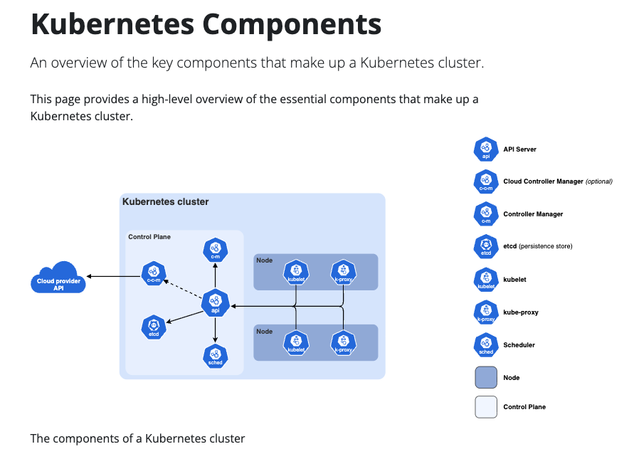
In deployment, the same motivation now appears as container orchestration, service meshes, distributed databases, event streams, globally replicated control planes, ML training clusters, inference fleets, edge services, and workflow systems. Kubernetes describes itself as an open-source system for automating deployment, scaling, and management of containerized applications, and its own architecture separates a control plane from worker nodes so that desired state can be declared, reconciled, and observed across a cluster; Kubernetes Components is the canonical reference for the API server, etcd, scheduler, controllers, kubelet, kube-proxy, and container runtime.
The following figure (source) shows the main Kubernetes cluster components, including the control plane, worker nodes, API server, scheduler, controllers, etcd, kubelet, kube-proxy, and container runtime.
The core problem: useful coordination without perfect knowledge
The central challenge is that no node has perfect global knowledge. A node knows its local state, messages it has received, local time according to its own clock, and any durable records it can read. It does not directly know whether another node has crashed, is slow, is partitioned, has processed a message, or has processed a newer message that has not yet arrived. This is why distributed systems are often designed around explicit state machines, durable logs, leases, idempotency keys, monotonic version numbers, quorums, heartbeats, failure detectors, and reconciliation loops.
A useful mental model is that distributed systems convert unreliable local observations into system-level guarantees. For example, a replicated log gives several machines the same ordered sequence of commands; a quorum protocol ensures that reads and writes overlap in at least one replica; a deployment controller keeps comparing actual state with desired state; and an event stream lets consumers recover from failure by replaying durable records. The Part-Time Parliament by Lamport (1998) introduced Paxos as a way for unreliable processes to agree on a value, while In Search of an Understandable Consensus Algorithm by Ongaro et al. (2014) presented Raft as an equivalent replicated-log consensus algorithm structured around leader election, log replication, and safety.
The basic tradeoffs
Distributed systems engineering is the management of tradeoffs. A design that improves one property often weakens another.
| Design pressure | Typical improvement | Typical cost |
|---|---|---|
| Replication | Higher read capacity, durability, and availability | Consistency complexity and write coordination |
| Sharding | Higher write capacity and storage scale | Cross-shard transactions and rebalancing complexity |
| Caching | Lower latency and lower backend load | Staleness and invalidation complexity |
| Consensus | Strong coordination and linearizable metadata | Higher write latency and reduced availability under partitions |
| Asynchronous messaging | Loose coupling and retryable workflows | Duplicate delivery, reordering, and eventual consistency |
| Global deployment | Lower user latency and regional resilience | Clock, consistency, compliance, and failover complexity |
| Microservices | Independent deployment and ownership | Network failure, observability, versioning, and dependency management |
| Automation | Faster recovery and safer rollout | Control-loop bugs and misconfigured policies |
The CAP theorem is often used to frame the consistency and availability tradeoff under network partition, but the useful production interpretation is narrower: when communication between replicas is disrupted, a replicated service must choose whether to reject some operations or risk serving non-single-copy behavior. Brewer’s Conjecture and the Feasibility of Consistent, Available, Partition-Tolerant Web Services by Gilbert et al. (2002) formalized this impossibility result, while Perspectives on the CAP Theorem by Gilbert et al. (2012) clarifies that real systems operate across a spectrum of consistency, latency, failure, and recovery modes rather than choosing a simplistic “two of three” label.
A small set of equations that appear repeatedly
Availability is usually stated as the fraction of time a service is able to handle requests successfully:
\[A = \frac{\text{uptime}}{\text{uptime} + \text{downtime}}.\]For independent replicas, the probability that at least one of \(n\) replicas is available is:
\[A_{\text{replicated}} = 1 - \prod_{i=1}^{n}(1 - A_i).\]This equation is idealized because real failures are often correlated, for example by shared power, shared software bugs, shared control planes, shared cloud regions, or shared dependencies. Still, it explains why replication helps most when replicas fail independently.
Quorum systems are usually described with \(N\) replicas, write quorum size \(W\), and read quorum size \(R\). A common condition for read-write quorum overlap is:
\[R + W > N.\]When this inequality holds, every read quorum intersects every write quorum in at least one replica, which gives the protocol a place to observe the latest completed write if versions and conflict rules are implemented correctly. Dynamo-style systems expose these quorum parameters as design knobs, and Dynamo: Amazon’s Highly Available Key-value Store by DeCandia et al. (2007) uses this style of replication, versioning, and reconciliation to provide high availability for core Amazon services.
Tail latency is often more important than mean latency. If a request fans out to \(k\) independent subrequests and each subrequest completes within latency threshold \(t\) with probability \(p\), then the probability that all subrequests complete within \(t\) is:
\[P(\max(X_1, X_2, \ldots, X_k) \leq t) = p^k.\]This is why high fanout systems can have bad end-to-end tail latency even when each individual service looks healthy. The Tail at Scale by Dean et al. (2013) explains why large online services must tolerate latency variability through techniques such as hedged requests, backup tasks, load balancing, and careful fanout control.
The implementation lens
A production distributed system is usually not a single algorithm. It is a composition of several implementation patterns:
- Nodes communicate through RPC, HTTP, gRPC, message queues, logs, gossip, or shared durable storage.
- State is kept in memory for speed, but authoritative state is placed in databases, logs, object stores, consensus-backed metadata stores, or append-only event streams.
- Replication is used for durability and availability, while sharding is used for scale.
- Idempotency, deduplication, sequence numbers, and transactional outboxes are used because retries are unavoidable.
- Health checks, leases, leader election, and heartbeats are used because failure detection is uncertain.
- Observability systems collect metrics, logs, traces, profiles, and events because no single node sees the whole system.
- Deployment systems use rolling updates, canaries, blue-green releases, feature flags, autoscaling, and rollback because software changes are among the most common causes of failure.
Google’s Borg, Omega, and Kubernetes by Burns et al. (2016) is especially useful for deployment thinking because it connects cluster management, declarative APIs, persistent cluster state, containers, health checks, autoscaling, service discovery, and rollout tooling into one operational model. The same lineage also explains why modern platforms treat infrastructure as an application-oriented control plane rather than as a collection of individually managed machines.
The main conceptual layers
A complete primer on distributed systems needs to move through several layers, because each layer depends on the one below it.
| Layer | Core question | Typical mechanisms |
|---|---|---|
| Models and failure assumptions | What can go wrong, and what does the system promise anyway? | Crash faults, Byzantine faults, partitions, timeouts, retries, partial synchrony |
| Time and ordering | What happened before what? | Logical clocks, vector clocks, hybrid logical clocks, timestamps, causal order |
| Communication | How do nodes exchange work and state? | RPC, queues, streams, pub-sub, gossip, backpressure |
| Replication | How is state copied safely? | Leader-follower replication, quorum replication, consensus, anti-entropy |
| Consistency | What can clients observe? | Linearizability, serializability, causal consistency, eventual consistency, read-your-writes |
| Partitioning | How is data or work split? | Hash partitioning, range partitioning, consistent hashing, resharding |
| Transactions and workflows | How are multi-step changes made safe? | Two-phase commit, sagas, outbox pattern, escrow, compensation |
| Storage systems | How is data stored and recovered? | LSM trees, WALs, snapshots, distributed filesystems, object stores |
| Compute systems | How is work scheduled and executed? | Batch jobs, stream processors, DAG schedulers, actors, serverless |
| Deployment platforms | How does code run in production? | Kubernetes, schedulers, service discovery, load balancing, rollouts |
| Reliability engineering | How is failure expected and managed? | SLOs, error budgets, incident response, chaos testing, graceful degradation |
| Security and multi-tenancy | How is trust bounded? | mTLS, identity, RBAC, network policy, secrets, isolation, audit logs |
Distributed systems as control loops
Modern deployment platforms are best understood as control loops. A user writes desired state, such as “run five replicas of this service,” and a controller repeatedly observes actual state, compares it with desired state, and takes actions to reduce the difference. Kubernetes documents this architecture through its API server, scheduler, controllers, etcd, kubelet, and node components; Kubernetes Components gives the concrete production decomposition.
A generic reconciliation loop looks like this:
while True:
    desired = read_desired_state()
    actual = observe_actual_state()

    diff = compare(desired, actual)

    for action in plan(diff):
        if action_is_safe(action):
            apply(action)

    sleep(reconcile_interval)
The hard parts are hidden inside the helpers. read_desired_state must be consistent enough to avoid split-brain behavior. observe_actual_state must handle stale or missing signals. plan must avoid oscillation. apply must be idempotent because the controller may crash after sending an action but before recording success. action_is_safe must encode rollout budgets, disruption budgets, quota, admission policy, dependency constraints, and security rules. This is why distributed systems work is often less about writing a single clever algorithm and more about specifying invariants, making side effects retry-safe, and ensuring that recovery paths are ordinary paths.
What “advanced” means in deployed systems
Advanced distributed systems are not merely systems that use Paxos, Raft, or global transactions. In deployed systems, advanced usually means the design handles scale, partial failure, operational change, and human error at the same time.
An advanced production system usually has:
- clear consistency contracts per API rather than one vague consistency label;
- explicit ownership of state, with durable logs or databases as recovery anchors;
- idempotent APIs and safe retry behavior;
- bounded queues, backpressure, and overload control;
- multi-zone or multi-region failure handling;
- automated rollout and rollback;
- structured observability around service-level indicators;
- capacity models and autoscaling policies;
- dependency isolation, graceful degradation, and circuit breaking;
- security boundaries for identity, authorization, encryption, and tenancy;
- disaster recovery plans tested through drills rather than assumed from diagrams.
Google’s SRE material is central for this operational layer. Monitoring Distributed Systems explains how monitoring should distinguish urgent human pages from non-urgent diagnostic information, and Service Level Objectives frames reliability through measurable SLIs, SLOs, and error budgets rather than vague uptime aspirations.
Primer roadmap
The rest of this primer will build from foundations to deployment practice:
- Foundations: system models, failures, clocks, ordering, and the impossibility results that define the design space.
- Communication: RPC, retries, idempotency, queues, streams, pub-sub, backpressure, and flow control.
- Replication and consensus: leader election, replicated logs, quorums, Paxos, Raft, leases, membership, snapshots, and reconfiguration.
- Consistency models: linearizability, serializability, sequential consistency, causal consistency, eventual consistency, session guarantees, and conflict resolution.
- Data partitioning: sharding, consistent hashing, range partitioning, hotspot mitigation, resharding, and placement.
- Distributed storage: WALs, LSM trees, distributed filesystems, object stores, metadata planes, compaction, repair, and backup.
- Transactions and workflows: two-phase commit, sagas, outbox, exactly-once boundaries, compensation, and long-running business processes.
- Compute systems: batch, stream processing, DAGs, actors, serverless, GPU clusters, and distributed ML workloads.
- Service architecture: microservices, service discovery, load balancing, API gateways, service meshes, and dependency management.
- Deployment infrastructure: containers, Kubernetes, scheduling, rollouts, autoscaling, configuration, secrets, multi-region deployment, and control planes.
- Reliability and operations: SLOs, observability, incident response, chaos engineering, overload, tail latency, capacity, and disaster recovery.
- Security and governance: identity, mTLS, authorization, isolation, policy, supply chain security, audit, and multi-tenancy.
- Advanced design patterns: CRDTs, local-first systems, active-active databases, edge systems, global databases, and large-scale AI-serving infrastructure.
Foundations
System model
A distributed system model defines what exists, how components communicate, what can fail, and what guarantees an algorithm is allowed to rely on. The most common model has processes, messages, local state, local clocks, and a network that can delay, reorder, duplicate, or drop messages depending on the assumed transport. Time, Clocks, and the Ordering of Events in a Distributed System by Lamport (1978) gives the classic formulation: a distributed system is a set of distinct processes that communicate by exchanging messages, and the key difficulty is that message delay is not negligible compared with local computation.
A process can observe its own local state and the messages it receives. It cannot directly observe another process’s local state, another process’s clock, the contents of the network, or whether a missing response means failure, delay, overload, packet loss, or a partition. This is why most distributed algorithms are written in terms of observable events: local computation, send events, receive events, durable writes, timeouts, and membership changes. Lamport’s paper is important because it formalizes the difference between physical time and observable causal order, which is the foundation for reasoning about correctness without a shared clock.
A minimal implementation model looks like this:
class Node:
    def __init__(self, node_id: str):
        self.node_id = node_id
        self.local_state = {}
        self.inbox = []
        self.outbox = []

    def on_message(self, message):
        # A receive event. This is the only point where remote information
        # becomes locally observable.
        self.apply(message)

    def send(self, destination: str, payload: dict):
        # A send event. The sender cannot assume when, whether, or how many
        # times the message will be observed by the receiver.
        self.outbox.append({
            "from": self.node_id,
            "to": destination,
            "payload": payload,
        })
The model matters because different assumptions lead to different algorithms. If the network is synchronous, an algorithm can rely on known bounds for message delay and processing time. If the network is asynchronous, there are no fixed timing bounds, so timeout-based conclusions are only guesses. Consensus in the Presence of Partial Synchrony by Dwork et al. (1988) introduced practically motivated models between full synchrony and full asynchrony, which is why many deployed systems are designed around eventual timing stability rather than perfect timing.
Safety and liveness
Most distributed guarantees can be split into safety and liveness. A safety property says that something bad never happens. A liveness property says that something good eventually happens. This distinction is central because many algorithms preserve safety during extreme failures but may temporarily lose liveness. Impossibility of Distributed Consensus with One Faulty Process by Fischer et al. (1985) shows that deterministic consensus cannot guarantee termination in a fully asynchronous system with even one crash-faulty process, which is a liveness impossibility rather than a safety impossibility.
Examples:
| Property | Type | Meaning |
|---|---|---|
| At most one leader is active for a term | Safety | The system must not create two conflicting authorities for the same epoch |
| Every committed log entry is preserved | Safety | A later leader cannot erase committed history |
| Every client request eventually receives a response | Liveness | The system continues making progress |
| Every non-faulty replica eventually catches up | Liveness | Replication eventually converges |
| No two successful withdrawals spend the same balance | Safety | The same funds cannot be committed twice |
| A queued job eventually runs | Liveness | The scheduler cannot starve work forever |
A practical system usually chooses safety first for critical state and relaxes liveness under uncertainty. For example, a consensus-backed metadata service may reject writes during a partition rather than accept conflicting leaders. A shopping cart service may accept writes locally and reconcile later because availability is more valuable than immediate single-copy consistency for that product surface. Dynamo: Amazon’s Highly Available Key-value Store by DeCandia et al. (2007) is a canonical example of choosing availability with versioned objects and application-level conflict resolution for a production key-value store.
A useful way to write design invariants is:
\[\text{safety}: \forall t,\ \neg \text{bad}(S_t)\] \[\text{liveness}: \exists t' > t,\ \text{good}(S_{t'})\]The implementation implication is that monitoring only “is the system up?” is insufficient. Operators also need checks for invariant violations, stale progress, stuck queues, leader churn, replication lag, and divergence. Jepsen is useful here because it tests whether distributed databases, queues, and consensus systems actually satisfy their documented safety claims under faults.
Failure models
Failure models specify what kinds of faults the system is expected to tolerate. A crash fault means a process stops executing. An omission fault means messages may be lost or not sent. A timing fault means responses arrive too late for the system’s assumptions. A Byzantine fault means a process can behave arbitrarily, including lying, equivocating, or colluding. Most web infrastructure assumes crash or omission faults; blockchains, some replicated ledgers, and adversarial multi-party systems use Byzantine fault-tolerant protocols.
| Failure type | Example | Common mitigation |
|---|---|---|
| Crash fault | A process exits or a VM disappears | Replication, restart, leader election |
| Omission fault | A message is dropped | Retries, durable queues, acknowledgments |
| Timing fault | A dependency responds after the timeout | Deadlines, hedging, backpressure |
| Partition | Two groups of nodes cannot communicate | Quorum rules, failover policy, degraded mode |
| Data corruption | Disk or memory returns bad data | Checksums, replicas, scrubbers |
| Byzantine fault | A node sends conflicting messages | Signatures, quorum certificates, BFT consensus |
| Operator fault | A bad config is rolled out | Staged rollout, policy checks, rollback |
| Correlated fault | All replicas share a buggy binary | Diversity, canaries, blast-radius limits |
A failure detector is the part of a system that suspects whether another process has failed. In a real asynchronous network, a failure detector cannot distinguish a crashed process from a slow or partitioned process with certainty. Unreliable Failure Detectors for Reliable Distributed Systems by Chandra et al. (1996) introduced failure detectors as formal abstractions and classified them by completeness and accuracy, which maps directly to production concepts like heartbeats, suspicions, and eventually-correct membership.
A simple heartbeat detector illustrates the idea:
import time

class FailureDetector:
    def __init__(self, timeout_seconds: float):
        self.timeout_seconds = timeout_seconds
        self.last_seen = {}

    def heartbeat_received(self, node_id: str) -> None:
        self.last_seen[node_id] = time.monotonic()

    def suspected_failed(self, node_id: str) -> bool:
        last = self.last_seen.get(node_id)
        if last is None:
            return True
        return time.monotonic() - last > self.timeout_seconds
This detector is intentionally unreliable. It can falsely suspect a healthy node if the node is slow, the network is congested, the runtime is paused by garbage collection, the host is overloaded, or the detector itself is delayed. Production systems therefore treat suspicion as an input to a protocol, not as proof. A leader election protocol may require a quorum before acting on suspicion; a load balancer may remove a backend temporarily; a deployment controller may wait for several failed probes before restarting a pod.
Network assumptions and the fallacies of distributed computing
Distributed systems fail when code assumes the network behaves like local memory. The “fallacies of distributed computing” are a compact list of false assumptions often attributed to L. Peter Deutsch and others at Sun Microsystems: the network is reliable, latency is zero, bandwidth is infinite, the network is secure, topology does not change, there is one administrator, transport cost is zero, and the network is homogeneous. The list is summarized in Fallacies of distributed computing, and it remains useful as an engineering checklist even though it is not a formal theorem.
The implementation consequence is that every remote call needs a policy:
def call_remote_service(request, *, deadline, idempotency_key):
    try:
        return rpc_call(
            request=request,
            timeout=deadline.remaining(),
            headers={"Idempotency-Key": idempotency_key},
        )
    except TimeoutError:
        # Unknown outcome: the server may have processed the request.
        # Only retry safely if the operation is idempotent or deduplicated.
        return retry_or_surface_unknown(request, idempotency_key)
    except ConnectionError:
        # Likely not processed, but still not guaranteed.
        return retry_with_backoff(request, idempotency_key)
The important detail is the “unknown outcome” state. If a client times out after sending a payment request, the client does not know whether the payment service received and committed it. The safe implementation is not “retry blindly,” but “retry with an idempotency key against an endpoint that deduplicates by that key.” This pattern appears in payment systems, job queues, workflow engines, database clients, object storage writes, and deployment controllers.
A robust remote operation generally needs:
| Concern | Implementation detail |
|---|---|
| Timeout | Every call has a deadline; no unbounded waits |
| Retry | Retries use exponential backoff and jitter |
| Deduplication | Mutating requests carry idempotency keys |
| Ordering | Sequence numbers or versions reject stale writes |
| Backpressure | Callers stop sending when queues or dependencies are overloaded |
| Circuit breaking | Repeated failures temporarily stop traffic to a dependency |
| Observability | Every request carries trace IDs and structured error information |
Time, clocks, and causality
Physical clocks are useful for logs, leases, metrics, user-facing timestamps, and approximate ordering, but they are not a perfect source of truth. Clocks can drift, jump, be misconfigured, or disagree across hosts. Lamport’s key insight was that causality can be modeled without relying on synchronized physical clocks. Time, Clocks, and the Ordering of Events in a Distributed System by Lamport (1978) defines the “happened-before” relation and shows that it forms a partial order over events.
The following figure (source) shows Lamport’s process-time diagrams for events and messages, where vertical process lines, event points, and message arrows define a partial causal order rather than a single global timeline.
The happened-before relation is usually written as:
\[a \rightarrow b\]It is defined by three rules:
\[\text{If } a \text{ and } b \text{ occur in the same process and } a \text{ comes before } b,\ \text{then } a \rightarrow b.\] \[\text{If } a \text{ is the send of a message and } b \text{ is the receive of that message,\ then } a \rightarrow b.\] \[\text{If } a \rightarrow b \text{ and } b \rightarrow c,\ \text{then } a \rightarrow c.\]If neither event happened before the other, the events are concurrent:
\[a \parallel b \iff \neg(a \rightarrow b) \land \neg(b \rightarrow a)\]This matters in implementation because two writes that arrive in different orders at different replicas may not have a causal relationship. Treating them as if one “really came first” can create incorrect conflict resolution. Systems that need to preserve causality use logical clocks, vector clocks, dependency metadata, session guarantees, or transactions.
Lamport clocks
A Lamport clock assigns a monotonically increasing integer timestamp to each event. The guarantee is one-way: if event \(a\) happened before event \(b\), then the Lamport timestamp of \(a\) is smaller than the Lamport timestamp of \(b\). The converse is not guaranteed, because two concurrent events can still receive ordered timestamps. Time, Clocks, and the Ordering of Events in a Distributed System by Lamport (1978) gives the original logical-clock rules and explains how they can extend a partial order into a total order by adding deterministic tie-breaking.
The clock condition is:
\[a \rightarrow b \implies C(a) < C(b)\]A simple implementation is:
class LamportClock:
    def __init__(self):
        self.time = 0

    def tick(self) -> int:
        self.time += 1
        return self.time

    def send_timestamp(self) -> int:
        return self.tick()

    def receive_timestamp(self, remote_time: int) -> int:
        self.time = max(self.time, remote_time) + 1
        return self.time
A message includes the sender’s timestamp:
def send(clock: LamportClock, payload: dict) -> dict:
    return {
        "timestamp": clock.send_timestamp(),
        "payload": payload,
    }

def receive(clock: LamportClock, message: dict) -> None:
    clock.receive_timestamp(message["timestamp"])
    apply(message["payload"])
Lamport clocks are useful when a system needs deterministic ordering but does not need to know whether two events were truly concurrent. Examples include ordering replicated log candidates, producing sortable event IDs, debugging traces, and implementing simple last-writer-wins logic with a tie-breaker. They are insufficient when the application must detect concurrency, because \(C(a) < C(b)\) does not prove \(a \rightarrow b\).
Vector clocks
Vector clocks extend logical clocks by keeping one counter per process. They can detect whether one event causally precedes another or whether two events are concurrent. Timestamps in Message-Passing Systems That Preserve the Partial Ordering by Fidge (1988) and related work by Mattern introduced vector-clock mechanisms for preserving partial order in message-passing systems; Timestamping Messages and Events in a Distributed System by Garg (2007) summarizes the mechanism and its cost of maintaining a vector of size \(N\) for \(N\) processes.
For a system with \(N\) nodes, node \(i\) maintains:
\[V_i = [v_1, v_2, \ldots, v_N]\]On a local event at node \(i\):
\[V_i[i] \leftarrow V_i[i] + 1\]On send, the message carries \(V_i\). On receive at node \(j\):
\[V_j[k] \leftarrow \max(V_j[k], V_{\text{msg}}[k])\ \text{for all } k\] \[V_j[j] \leftarrow V_j[j] + 1\]One vector is causally before another if every component is less than or equal and at least one component is strictly less:
\[V(a) < V(b) \iff \left(\forall k,\ V(a)_k \leq V(b)_k\right) \land \left(\exists k,\ V(a)_k < V(b)_k\right)\]Two events are concurrent if neither vector dominates the other:
\[V(a) \parallel V(b) \iff \neg(V(a) < V(b)) \land \neg(V(b) < V(a))\]A compact implementation is:
class VectorClock:
    def __init__(self, node_id: str, all_nodes: list[str]):
        self.node_id = node_id
        self.clock = {node: 0 for node in all_nodes}

    def tick(self) -> dict[str, int]:
        self.clock[self.node_id] += 1
        return dict(self.clock)

    def send_timestamp(self) -> dict[str, int]:
        return self.tick()

    def receive_timestamp(self, remote: dict[str, int]) -> dict[str, int]:
        for node, value in remote.items():
            self.clock[node] = max(self.clock.get(node, 0), value)
        self.clock[self.node_id] += 1
        return dict(self.clock)

def compare(a: dict[str, int], b: dict[str, int]) -> str:
    nodes = set(a) | set(b)
    a_le_b = all(a.get(n, 0) <= b.get(n, 0) for n in nodes)
    b_le_a = all(b.get(n, 0) <= a.get(n, 0) for n in nodes)
    a_lt_b = a_le_b and any(a.get(n, 0) < b.get(n, 0) for n in nodes)
    b_lt_a = b_le_a and any(b.get(n, 0) < a.get(n, 0) for n in nodes)

    if a_lt_b:
        return "a_before_b"
    if b_lt_a:
        return "b_before_a"
    return "concurrent"
Vector clocks are useful in eventually consistent stores, collaborative systems, anti-entropy protocols, debugging, and conflict detection. Their main cost is metadata growth: a full vector has size \(O(N)\), which is expensive when the number of writers is large or dynamic. Production systems often use dotted version vectors, version vectors scoped to replicas, hybrid logical clocks, or application-level conflict rules to reduce this overhead.
Physical clocks, leases, and clock skew
Physical clocks are still widely used, but only under explicit error bounds. A lease is a time-bounded authority, for example “this node may act as leader until time \(T\).” Leases are attractive because they can reduce coordination after acquisition, but they are dangerous if clock skew is ignored. If one node’s clock runs slow and another node’s clock runs fast, both may believe they hold a valid lease unless the protocol accounts for maximum skew and renewal timing.
A simple lease safety rule is:
\[T_{\text{holder-expiry}} + \epsilon < T_{\text{observer-now}}\]where \(\epsilon\) is a conservative bound on clock uncertainty. This means an observer should not assume a remote lease has expired until enough time has passed to account for skew. Lamport’s paper includes a physical-clock synchronization section and derives bounds on how far clocks can drift under assumptions about message delay and clock rates, which is the conceptual basis for using physical time only when its uncertainty is modeled. Time, Clocks, and the Ordering of Events in a Distributed System by Lamport (1978) is therefore relevant both for logical clocks and for bounded physical-clock reasoning.
A lease implementation should include fencing tokens. A fencing token is a monotonically increasing number issued when a lease is acquired. Downstream systems reject stale tokens even if an old leader wakes up and tries to write.
class LeaseStore:
    def __init__(self):
        self.owner = None
        self.expiry_ms = 0
        self.fencing_token = 0

    def try_acquire(self, node_id: str, now_ms: int, ttl_ms: int):
        if now_ms >= self.expiry_ms:
            self.fencing_token += 1
            self.owner = node_id
            self.expiry_ms = now_ms + ttl_ms
            return {
                "granted": True,
                "fencing_token": self.fencing_token,
                "expiry_ms": self.expiry_ms,
            }
        return {"granted": False}

class FencedResource:
    def __init__(self):
        self.last_token = 0

    def write(self, token: int, value: str):
        if token < self.last_token:
            raise ValueError("stale lease holder")
        self.last_token = token
        persist(value)
The key deployment point is that a lease alone is not enough. The resource being protected must enforce the fencing token, otherwise a paused process can resume after its lease expires and still perform unsafe writes.
Global state and distributed snapshots
A global state is the combination of all process states and all in-flight channel states. Since distributed systems usually do not have a shared clock, it is not possible to simply ask every node to “record the state at exactly 12:00:00.” Distributed Snapshots: Determining Global States of Distributed Systems by Chandy et al. (1985) introduced an algorithm for recording a meaningful global state while the underlying computation continues, using marker messages to separate pre-snapshot and post-snapshot traffic.
The following figure (source) shows a simple distributed system with two processes, two channels, and a token whose location defines the global state, illustrating why a snapshot must include both process state and channel state.
![]()
The Chandy-Lamport snapshot algorithm assumes reliable FIFO channels. In simplified form:
class SnapshotNode:
    def __init__(self, node_id, outgoing_channels):
        self.node_id = node_id
        self.outgoing_channels = outgoing_channels
        self.recorded = False
        self.local_snapshot = None
        self.channel_snapshots = {}

    def start_snapshot(self, snapshot_id):
        self.recorded = True
        self.local_snapshot = self.record_local_state()

        for channel in self.outgoing_channels:
            channel.send({
                "type": "MARKER",
                "snapshot_id": snapshot_id,
            })

    def on_marker(self, snapshot_id, from_channel):
        if not self.recorded:
            self.recorded = True
            self.local_snapshot = self.record_local_state()
            self.channel_snapshots[from_channel] = []

            for channel in self.outgoing_channels:
                channel.send({
                    "type": "MARKER",
                    "snapshot_id": snapshot_id,
                })
        else:
            # Messages received on this channel before the marker are part of
            # the channel state. After the marker, this channel is closed for
            # this snapshot.
            self.close_channel_snapshot(from_channel, snapshot_id)

    def on_application_message(self, message, from_channel):
        if self.recorded and not self.channel_snapshot_closed(from_channel):
            self.channel_snapshots[from_channel].append(message)

        self.apply(message)
The snapshot algorithm is foundational for checkpointing, termination detection, deadlock detection, stream processing checkpoints, and consistent backup. Its main lesson is that “global state” is not a variable sitting somewhere. It is a constructed view assembled from local states and in-flight messages under a consistency rule. In production, similar ideas appear in stream processors that align barriers across input partitions, databases that coordinate snapshots with log positions, and backup systems that combine object snapshots with metadata checkpoints.
Consensus and the FLP boundary
Consensus is the problem of getting multiple processes to agree on one value. A consensus protocol usually requires agreement, validity, and termination. Agreement means correct processes do not decide different values. Validity means the decided value came from an allowed proposal. Termination means correct processes eventually decide.
The FLP result defines a hard boundary: in a fully asynchronous system, no deterministic consensus protocol can guarantee termination if even one process may crash. Impossibility of Distributed Consensus with One Faulty Process by Fischer et al. (1985) is the standard reference, and its practical significance is that consensus protocols need some extra assumption, such as timing assumptions, randomization, failure detectors, stable storage, or operational limits.
This does not mean consensus is impossible in practice. It means production consensus systems are not purely asynchronous mathematical objects. They use timeouts to suspect leaders, quorums to preserve safety, randomized or term-based elections to avoid repeated collisions, and eventually stable network assumptions to regain liveness. Consensus in the Presence of Partial Synchrony by Dwork et al. (1988) is important because it explains the middle ground where systems can be asynchronous for some period but eventually behave synchronously enough for progress.
A simplified consensus interface hides enormous complexity:
class ConsensusLog:
    def propose(self, command: dict) -> int:
        """
        Append command to a replicated log and return its committed index.
        Safety requirement:
        once an index is committed, no different command can be committed
        at that index.
        """
        raise NotImplementedError

    def read_committed(self, index: int) -> dict:
        raise NotImplementedError
The core invariant for replicated logs is:
\[\text{If two correct replicas commit entries at index } i,\ \text{then those entries are identical.}\]Consensus is normally used for small, high-value coordination state: cluster membership, leader election, metadata, locks, configuration, schema changes, and replicated logs. It is usually not used for every data-plane request in a high-throughput system unless strong consistency is required, because quorum coordination adds latency and reduces availability during partitions.
CAP and PACELC
The CAP theorem applies to replicated shared-data systems under network partition. In a partition, a system that continues accepting operations on both sides may sacrifice single-copy consistency, while a system that preserves single-copy consistency must reject or block some operations. Brewer’s Conjecture and the Feasibility of Consistent, Available, Partition-Tolerant Web Services by Gilbert et al. (2002) formalized the result; CAP Twelve Years Later: How the “Rules” Have Changed by Brewer (2012) is useful because it explains why the simplistic “pick two” framing is misleading in real systems.
PACELC extends the operational framing: if there is a partition, choose between availability and consistency; else, during normal operation, choose between latency and consistency. Consistency Tradeoffs in Modern Distributed Database System Design by Abadi (2012) is the standard PACELC reference, and its relevant point is that the latency-consistency tradeoff exists even when the network is healthy.
The practical reading is:
| Situation | Design question |
|---|---|
| Partition exists | Should the system reject some operations or accept divergent writes? |
| No partition | Should the system coordinate before responding or serve from a nearby replica? |
A common mistake is to label an entire system as “CP” or “AP.” Real systems often make different choices per operation. For example, a database may require consensus for schema changes, quorum writes for critical records, local reads for cached profiles, and asynchronous replication for analytics events. A deployment platform may use a strongly consistent metadata store for desired state while allowing eventually consistent node status updates.
Consistency vocabulary at the foundation layer
Consistency models define what clients are allowed to observe. The details will be covered later, but the foundations matter early because consistency is not one thing. Linearizability gives the illusion that each operation takes effect atomically at some instant between invocation and response. Serializability says transactions behave like some serial order, but not necessarily one that respects real-time order. Causal consistency preserves happened-before relationships. Eventual consistency says replicas converge if updates stop, but does not by itself specify what intermediate states clients may observe. Consistency Models is a useful engineering reference because it organizes these models by the histories they permit and the anomalies they rule out.
A simple way to connect models to implementation:
| Model | Implementation tendency | Cost |
|---|---|---|
| Linearizability | Leader, consensus, quorum read/write, leases with fencing | Higher latency and lower partition availability |
| Serializability | Transaction scheduler, optimistic concurrency control, two-phase locking, MVCC | Coordination or aborts under contention |
| Causal consistency | Dependency tracking, vector clocks, session metadata | Metadata and dependency management |
| Eventual consistency | Async replication, anti-entropy, conflict resolution | Temporary anomalies and application-level reconciliation |
The important foundation is that consistency is a contract, not a storage engine feature name. A system should state which operations are linearizable, which are read-your-writes, which are eventually consistent, and which are best-effort. Without that contract, clients build accidental assumptions that break under failover, replication lag, retries, or deployment changes.
Idempotency, retries, and duplicate-safe design
Retries are mandatory because networks and processes fail. But retries turn every operation into a possible duplicate. A mutating operation is safe to retry only if the server can detect duplicates or the operation is naturally idempotent. This is one of the most important implementation foundations for production systems.
An operation is idempotent if applying it multiple times has the same effect as applying it once:
\[f(f(x)) = f(x)\]Examples:
| Operation | Idempotent? | Reason |
|---|---|---|
| Set user status to “inactive” | Yes | Repeating the same assignment does not change the result |
| Increment balance by \(10\) | No | Repeating increments changes the result |
| Create order with idempotency key \(K\) | Yes, if deduplicated | Repeating returns the original order |
| Send email | No, unless deduplicated | Repeating may send multiple emails |
| Mark job complete with version check | Yes, if guarded | Stale or duplicate completions are rejected |
A common server-side pattern:
class IdempotencyStore:
    def __init__(self):
        self.results_by_key = {}

    def run_once(self, key: str, operation):
        if key in self.results_by_key:
            return self.results_by_key[key]

        result = operation()
        self.results_by_key[key] = result
        return result

def create_order(request):
    key = request.headers["Idempotency-Key"]

    return idempotency_store.run_once(
        key,
        lambda: persist_order_and_charge(request),
    )
The subtle detail is atomicity. The idempotency record and the side effect must be committed together, or the system can crash after doing the side effect but before recording the key. Production implementations usually store the idempotency key in the same database transaction as the business mutation, or use an outbox pattern when a local transaction must trigger an external message.
Monotonicity and version checks
Many distributed races can be handled by making state transitions monotonic. A monotonic value moves in only one direction, such as increasing sequence numbers, increasing epochs, append-only log indexes, or state machines whose transitions do not go backward. Monotonicity is valuable because stale messages can be rejected without needing perfect timing.
A standard version-guarded write looks like this:
def update_if_version_matches(record_id: str, expected_version: int, patch: dict):
    record = db.get(record_id)

    if record.version != expected_version:
        raise ConflictError({
            "current_version": record.version,
            "expected_version": expected_version,
        })

    record.apply(patch)
    record.version += 1
    db.put(record)
    return record
The corresponding invariant is:
\[\text{accepted write at version } v \implies \text{current version before write was } v\]This pattern appears as compare-and-swap, optimistic concurrency control, generation numbers, Kubernetes resourceVersion, object-store conditional writes, database row versions, and fencing tokens. It is one of the simplest ways to avoid lost updates and stale-controller writes.
Membership and epochs
A distributed system needs to know which nodes are currently part of a group. Membership is difficult because joining, leaving, crashing, restarting, and partitioning can all happen concurrently. Production systems usually attach an epoch, term, generation, or configuration number to authority. A node’s message is accepted only if its epoch is current.
A simplified epoch check:
class Membership:
    def __init__(self):
        self.current_epoch = 0
        self.members = set()

    def install_configuration(self, epoch: int, members: set[str]):
        if epoch <= self.current_epoch:
            raise ValueError("stale membership update")

        self.current_epoch = epoch
        self.members = set(members)

    def validate_message(self, message):
        if message["epoch"] != self.current_epoch:
            raise ValueError("message from stale epoch")
        if message["from"] not in self.members:
            raise ValueError("sender is not a current member")
Epochs are essential for leader election, configuration changes, storage primaries, shard ownership, deployment controllers, and schedulers. Without epochs, an old leader can continue issuing commands after a new leader has taken over. With epochs but no fencing at the resource layer, an old leader can still cause damage. The implementation pattern is therefore: every authority has an epoch, every side effect carries that epoch or fencing token, and every protected resource rejects stale epochs.
Backpressure and bounded queues
A distributed system must handle overload explicitly. If every component retries aggressively while queues are growing, the system can enter a retry storm where extra recovery traffic makes the outage worse. Backpressure means the receiver communicates that it cannot accept unlimited work, and the sender slows down, sheds load, or degrades.
A bounded queue is the simplest form:
class BoundedQueue:
    def __init__(self, max_size: int):
        self.max_size = max_size
        self.items = []

    def offer(self, item) -> bool:
        if len(self.items) >= self.max_size:
            return False
        self.items.append(item)
        return True
A service should prefer explicit rejection over unbounded memory growth:
def handle_request(request):
    accepted = work_queue.offer(request)

    if not accepted:
        return {
            "status": 503,
            "retry_after_ms": 500,
            "error": "server overloaded",
        }

    return {"status": 202}
The deeper point is that queues hide latency. A service can appear healthy while queueing seconds or minutes of work. A production system should track queue depth, oldest item age, processing rate, retry rate, and drop rate. The Tail at Scale by Dean et al. (2013) is useful here because it explains how latency variability compounds in large fanout systems and motivates techniques such as hedged requests, backup tasks, and careful load control.
Partial failure as the default
Partial failure means one part of the system fails while other parts continue running. This is the normal state of large deployments. A single request might hit a healthy API server, a slow cache, a partitioned database replica, a degraded downstream service, and a successful logging pipeline at the same time. The application must decide what to do with partial results.
A practical policy table:
| Dependency | Failure behavior | Example |
|---|---|---|
| Authentication | Fail closed | Reject if identity cannot be verified |
| Payment authorization | Fail closed | Do not ship goods without authorization |
| Recommendation service | Fail open | Show fallback recommendations |
| Metrics pipeline | Fail open with buffering | Do not fail user requests because metrics failed |
| Search index | Degrade | Use stale index or limited search |
| Primary database | Fail over or reject | Depends on consistency contract |
This is a foundation because it changes API design. A service should not only define success and failure; it should define degraded success, retryable failure, permanent failure, unknown outcome, and compensation path.
What every production design should specify
A distributed design is incomplete unless it states its assumptions and invariants. At minimum, a production design should specify:
- Failure model: crash-only, omission, Byzantine, operator error, correlated regional failure, or some combination.
- Timing model: synchronous, asynchronous, partially synchronous, bounded clock skew, or best-effort physical time.
- Consistency contract: linearizable, serializable, causal, read-your-writes, monotonic reads, eventual, or per-operation.
- Durability contract: when data is acknowledged, where it is persisted, and how many failures it can survive.
- Retry contract: which operations are idempotent, how deduplication works, and what happens after unknown outcomes.
- Membership contract: how nodes join, leave, become leaders, lose authority, and reject stale epochs.
- Backpressure contract: what happens when queues, threads, memory, or downstream dependencies saturate.
- Recovery contract: how state is rebuilt after crash, restart, resharding, restore, failover, or replay.
- Observability contract: which metrics, logs, traces, events, and invariants prove the system is healthy.
- Operational contract: how deploys, rollbacks, migrations, config changes, and disaster recovery are performed.
The foundation of distributed systems is therefore not one algorithm. It is a disciplined way to reason about local knowledge, uncertain communication, partial failure, time, causality, retries, and invariants. Once these foundations are clear, replication, consensus, transactions, storage, compute, and deployment systems become easier to understand because each is a different way of enforcing useful guarantees under imperfect information.
Communication
Why communication is the first practical distributed-systems problem
Distributed systems are built from nodes that interact by sending messages. Those messages may be synchronous RPCs, asynchronous queue messages, append-only log records, pub-sub events, gossip updates, control-plane watch notifications, or telemetry spans. The communication layer determines latency, failure behavior, retry safety, ordering, backpressure, observability, and deployment coupling. In practice, many “distributed systems bugs” are communication bugs: a request timed out after the server committed it, a retry duplicated a side effect, a queue hid overload until latency exploded, a consumer committed an offset before processing was durable, a schema change broke an old consumer, or a trace lost its parent context across a queue boundary.
A local function call has one failure domain: either the process executes it or the process fails. A remote call has at least three: the caller, the network, and the callee. This is why remote communication must always specify a timeout, retry policy, idempotency contract, serialization format, authentication context, cancellation behavior, and observability metadata. RFC 9110: HTTP Semantics is useful for API design because it defines safe and idempotent HTTP method semantics, while Deadlines explains why gRPC clients should set explicit deadlines and why servers should stop work when the initiating RPC is cancelled.
The communication spectrum
Communication patterns range from tightly coupled request-response calls to loosely coupled durable event streams.
| Pattern | Typical interface | Coupling | Main advantage | Main risk |
|---|---|---|---|---|
| RPC | call service method and wait | High | Simple mental model and direct response | Timeout ambiguity and cascading failure |
| REST over HTTP | request resource and response | Medium | Universal tooling and cache-aware semantics | Verb misuse and unclear idempotency |
| Message queue | enqueue work, worker consumes | Medium-low | Buffering, retries, worker decoupling | Duplicate delivery and hidden backlog |
| Pub-sub | publish event to many subscribers | Low | Fanout and independent consumers | Schema drift and weak end-to-end ownership |
| Durable log or stream | append record, consumers track offsets | Low | Replay, ordering per partition, event history | Partitioning, lag, and offset correctness |
| Gossip | periodic peer-to-peer state exchange | Low | Scalable dissemination and failure detection | Eventual convergence and weak ordering |
| Watch API | subscribe to state changes | Medium | Efficient control-plane updates | Missed events unless paired with versioned state |
The choice should be driven by the business invariant, not by fashion. User-facing read paths often use synchronous RPC because the caller needs an answer now. Background work often uses queues because the caller only needs durable acceptance. Data integration, analytics, state replication, and event-driven architectures often use logs because consumers need replayable history. The Log: What every software engineer should know about real-time data’s unifying abstraction explains the log as an append-only ordered record of what happened, and its most relevant idea here is that a log provides both ordering and distribution for downstream systems.
Synchronous RPC
Synchronous RPC makes a remote operation look like a local function call, but it should not be treated like one. The caller must assume that any request can fail before send, fail during send, reach the server and fail during processing, succeed on the server but fail before the response reaches the caller, or complete too late to be useful. gRPC describes itself as a high-performance RPC framework with support for load balancing, tracing, health checking, and authentication, but the reliability behavior still depends on explicit deadlines, cancellation, retry policy, and service contracts. gRPC provides the general RPC model, and Deadlines is the key operational page because it states that clients have no default deadline and should set realistic ones.
A production RPC client should carry a request deadline instead of independent per-hop timeouts. A timeout says “wait at most \(x\) here.” A deadline says “the whole operation must finish by time \(T\).” Deadlines compose better because every downstream service can see the remaining budget:
\[\text{remaining_budget}*i = T*{\text{deadline}} - t_i.\]If the request path has \(n\) sequential hops, a naive independent timeout can exceed the caller’s intended limit:
\[T_{\text{worst}} = \sum_{i=1}^{n} t_i.\]A propagated deadline instead bounds the entire call graph:
\[T_{\text{end-to-end}} \leq T_{\text{deadline}} - T_{\text{start}}.\]A simple implementation pattern:
```python id=”grpc-deadline-budget” import time from dataclasses import dataclass
@dataclass(frozen=True) class RequestContext: trace_id: str deadline_monotonic: float idempotency_key: str | None = None
def remaining_seconds(self) -> float:
    return max(0.0, self.deadline_monotonic - time.monotonic())
def call_inventory_service(ctx: RequestContext, item_id: str) -> dict: remaining = ctx.remaining_seconds() if remaining <= 0: raise TimeoutError(“request deadline already expired”)
return grpc_call(
    method="Inventory/GetAvailability",
    payload={"item_id": item_id},
    timeout_seconds=remaining,
    metadata={
        "trace-id": ctx.trace_id,
        "idempotency-key": ctx.idempotency_key or "",
    },
) ```
The callee should also observe cancellation. If the client gives up, the server should stop expensive downstream work when correctness allows it. gRPC’s deadline documentation explicitly notes that servers may receive calls with unrealistic deadlines and that server applications are responsible for stopping work they started after cancellation.
```python id=”grpc-cancellation” def handle_search_request(request, ctx): for shard in choose_shards(request.query): if ctx.cancelled() or ctx.remaining_seconds() <= 0: raise RequestCancelled(“caller no longer needs this response”)
    partial = search_shard(
        shard=shard,
        query=request.query,
        timeout_seconds=ctx.remaining_seconds(),
    )
    merge(partial)

return build_response() ```
Remote-call outcome states
A remote mutation does not have only success and failure. It has success, known failure, retryable failure, permanent failure, and unknown outcome.
| Client observation | Server reality | Safe client behavior |
|---|---|---|
| Response received with success | Operation committed | Return success |
| Response received with validation error | Operation rejected before commit | Surface permanent failure |
| Connection failed before request send | Probably not processed | Retry if budget remains |
| Timeout after request send | Unknown | Retry only with idempotency or reconciliation |
| Server returned overloaded | Not processed or intentionally rejected | Retry later with backoff if allowed |
| Server crashed mid-request | Unknown | Retry only with idempotency or query state |
| Client crashed after response | Operation may be committed | Recover using durable request state |
The dangerous state is unknown outcome. For example, a payment request may have been committed even if the client timed out. Retrying without deduplication can double-charge. Not retrying can drop a valid user action. The server-side solution is to make the mutation idempotent by requiring a stable operation key and atomically storing the result for that key. HTTP’s formal idempotency definition is method-level, but application-level idempotency keys are needed for many POST-style business operations such as order creation, payment capture, and job submission. RFC 9110: HTTP Semantics defines idempotent request methods as methods whose intended server effect is the same after multiple identical requests as after one request.
```python id=”idempotent-rpc-server” def create_payment(request): key = request.headers[“Idempotency-Key”]
with db.transaction() as tx:
    previous = tx.query_one(
        "select response_json from idempotency where key = ?",
        [key],
    )
    if previous:
        return previous["response_json"]

    payment = tx.insert(
        "payments",
        {
            "account_id": request.account_id,
            "amount_cents": request.amount_cents,
            "status": "authorized",
        },
    )

    response = {
        "payment_id": payment["id"],
        "status": payment["status"],
    }

    tx.insert(
        "idempotency",
        {
            "key": key,
            "response_json": response,
        },
    )

    return response ```
The idempotency record must commit in the same transaction as the business state. Otherwise, the service can crash after authorizing the payment but before recording the idempotency key, which reintroduces the duplicate side effect.
Retries, backoff, jitter, and retry budgets
Retries are useful only when failures are transient and the operation is safe to repeat. Retrying too quickly can create a retry storm, where the recovery traffic becomes a new source of overload. Exponential Backoff And Jitter explains why exponential backoff alone is not enough under contention and why randomness spreads retry attempts across time; the relevant deployment lesson is that client libraries should avoid synchronized retry waves.
A common capped exponential backoff is:
\[d_i = \min(d_{\max}, d_0 \cdot 2^i)\]Full jitter samples uniformly from the backoff window:
\[d_i \sim U(0, \min(d_{\max}, d_0 \cdot 2^i)).\]A retry loop should also have a total deadline and a maximum attempt count:
```python id=”retry-backoff-jitter” import random import time
RETRYABLE_STATUS = {“UNAVAILABLE”, “RESOURCE_EXHAUSTED”, “DEADLINE_EXCEEDED”}
def call_with_retries(ctx, operation, *, max_attempts=4, base_delay=0.05, cap_delay=1.0): attempt = 0
while True:
    try:
        return operation(timeout_seconds=ctx.remaining_seconds())
    except RpcError as error:
        attempt += 1

        if error.status not in RETRYABLE_STATUS:
            raise

        if attempt >= max_attempts or ctx.remaining_seconds() <= 0:
            raise

        backoff = min(cap_delay, base_delay * (2 ** attempt))
        sleep_for = random.uniform(0, backoff)
        sleep_for = min(sleep_for, ctx.remaining_seconds())

        time.sleep(sleep_for) ```
Retries multiply load. If a service receives \(\lambda\) original requests per second and each request makes an expected \(E[A]\) attempts, the downstream receives:
\[\lambda_{\text{downstream}} = \lambda \cdot E[A].\]If each of \(k\) layers retries up to \(r\) times independently, the worst-case number of attempts against the deepest dependency can grow as:
\[A_{\max} = r^k.\]This is why production systems usually centralize retry policy at the edge or client library, cap attempts, respect deadlines, and avoid retrying non-idempotent mutations. Retry is useful because it distinguishes transparent retry from configured retry policy, and notes that gRPC only retries more aggressively when a retry policy allows it.
Hedging
Hedging sends a duplicate request before the original has failed, then uses the first successful response. It can reduce tail latency when slow requests are caused by transient queueing, noisy neighbors, or unlucky backend placement. It can also amplify load, so it should be limited to idempotent reads, bounded by deadlines, and triggered only after a delay based on observed latency percentiles. Request Hedging describes gRPC hedging as sending multiple copies of the same request to different backends and using the first response, with cancellation of outstanding attempts.
A typical policy is:
\[t_{\text{hedge}} = p_{95}(\text{latency})\]This means the client sends a second attempt only if the first attempt has already exceeded a high percentile for normal service time.
```python id=”hedged-read” def hedged_read(ctx, primary, backup, request, hedge_after_seconds): first = start_async(lambda: primary.read(request, timeout=ctx.remaining_seconds()))
if first.done_within(hedge_after_seconds):
    return first.result()

second = start_async(lambda: backup.read(request, timeout=ctx.remaining_seconds()))
winner = wait_first_success([first, second], timeout=ctx.remaining_seconds())

cancel_unfinished([first, second])
return winner ```
Hedging should not be used as a default fix for overload. If the backend is globally saturated, hedging makes the saturation worse.
Asynchronous messaging
Asynchronous messaging decouples producers from consumers by placing a broker, queue, or log between them. The producer can finish after durable enqueue, while consumers process later. This is useful for background jobs, slow integrations, burst absorption, fanout, workflow steps, and data pipelines. The cost is that the system now has eventual completion, duplicate delivery, dead-letter handling, ordering constraints, and operational lag.
A queue-based design usually has these components:
| Component | Role |
|---|---|
| Producer | Publishes a command, task, or event |
| Broker | Stores and delivers messages |
| Consumer | Processes messages and acknowledges success |
| Acknowledgement | Tells broker the message is safe to remove or mark complete |
| Negative acknowledgement | Tells broker the message was not processed |
| Dead-letter queue | Stores messages that repeatedly fail or expire |
| Retry policy | Controls delay and maximum attempts |
| Idempotency store | Prevents duplicate side effects |
RabbitMQ’s Consumer Acknowledgements and Publisher Confirms is a useful operational reference because it separates publisher confirms, which cover publisher-to-broker safety, from consumer acknowledgements, which cover broker-to-consumer processing safety. The important implementation detail is that these two acknowledgements are orthogonal, so a publisher confirm does not mean a consumer has processed the message.
```python id=”queue-consumer-ack” def consume_one(message): try: with db.transaction() as tx: if already_processed(tx, message.id): broker.ack(message) return
        process_business_effect(tx, message.payload)
        mark_processed(tx, message.id)

    broker.ack(message)

except RetryableError:
    broker.nack(message, requeue=True)

except PermanentError:
    broker.publish("dead-letter.orders", message)
    broker.ack(message) ```
The acknowledgement should happen after the business effect is durable. If the consumer acknowledges before committing, a crash can lose work. If the consumer commits before acknowledging, a crash can duplicate delivery. Therefore, consumers must be idempotent.
Delivery semantics
Messaging systems are often described using at-most-once, at-least-once, and exactly-once delivery. These terms are easy to misuse because they may refer to broker delivery, consumer processing, producer publishing, or end-to-end business effects.
| Semantics | Meaning | Typical failure mode |
|---|---|---|
| At-most-once | Message is delivered zero or one times | Data can be lost |
| At-least-once | Message is delivered one or more times | Duplicates can occur |
| Exactly-once broker pipeline | Broker avoids duplicate records within a defined transactional scope | External side effects may still duplicate |
| Exactly-once business effect | The real-world effect happens once | Requires idempotency, transactions, or reconciliation |
End-to-end exactly-once behavior is usually an application-level property, not just a broker feature. If a consumer reads a message, writes to an external payment API, and then commits an offset, the broker cannot prove whether the external payment happened once. This is why communication design usually combines at-least-once delivery with idempotent consumers. Pattern: Idempotent Consumer gives the practical pattern: record processed message IDs so duplicate deliveries can be detected and discarded.
A common invariant is:
\[\forall m,\ \text{business_effect}(m) \text{ is committed at most once}.\]One implementation uses a uniqueness constraint:
```sql id=”processed-message-table” create table processed_messages ( subscriber_id text not null, message_id text not null, processed_at timestamp not null default current_timestamp, primary key (subscriber_id, message_id) );
```python id="idempotent-consumer"
def handle_message(subscriber_id, message):
    with db.transaction() as tx:
        inserted = tx.try_insert(
            "processed_messages",
            {
                "subscriber_id": subscriber_id,
                "message_id": message.id,
            },
        )

        if not inserted:
            return "duplicate_ignored"

        apply_business_update(tx, message)

    return "processed"
Durable logs and streams
A durable log is an append-only sequence of records. A queue usually hides completed messages from consumers, while a log retains records for some time or size window and lets consumers track their own position. This is why logs are useful for replay, fanout, event sourcing, stream processing, CDC, analytics ingestion, and rebuilding derived state.
Kafka: a Distributed Messaging System for Log Processing by Kreps et al. (2011) introduced Kafka as a distributed messaging system for high-volume log data with low latency, and the most relevant design portions here are partitioned logs, pull-based consumption, consumer-managed offsets, batching, and per-partition ordering. The Apache Kafka documentation describes Kafka as a distributed, partitioned, replicated commit log service, and its documentation frames producers, brokers, topics, and consumers as the core communication model.
The following figure (source) shows Figure 1, Kafka Architecture, where producers publish to a cluster of brokers and consumers pull topic partitions from those brokers.
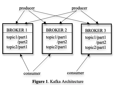
Kafka’s key abstraction is a topic partition. A topic is split into partitions, each partition is an ordered log, and each record has an offset within its partition. Consumers in the same consumer group divide partitions among themselves, while different consumer groups can independently consume the same topic. The original Kafka paper notes that a consumer consumes sequentially from a particular partition, that acknowledging an offset implies receipt of earlier messages in that partition, and that Kafka guarantees order within one partition but not across different partitions.
A simplified log model:
\[P_j = [r_{j,0}, r_{j,1}, \ldots, r_{j,n}]\]where \(P_j\) is partition \(j\) and \(r_{j,k}\) is the record at offset \(k\).
A consumer group state is a map:
\[O(g, t, p) = \text{next offset to read for group } g \text{ on topic } t \text{ partition } p.\]The current Kafka consumer-design documentation describes offsets as bookmarks for where a consumer group should resume, and notes that offsets are stored separately so consumers can recover after failure. Kafka Consumer Design is useful for the modern consumer-group and offset model.
Offset management
Offset commits define the failure semantics of stream consumption. If a consumer commits the offset before processing, a crash can skip the message. If a consumer processes first and commits later, a crash can reprocess the message. Most systems choose process-then-commit, which gives at-least-once processing and requires idempotent effects.
```python id=”stream-process-commit” def consume_partition(consumer, partition): while True: batch = consumer.poll(partition=partition, max_records=500)
    if not batch:
        continue

    with db.transaction() as tx:
        for record in batch:
            if not already_processed(tx, record.topic, record.partition, record.offset):
                apply_record(tx, record)
                mark_processed(tx, record.topic, record.partition, record.offset)

        next_offset = batch[-1].offset + 1
        store_consumer_offset(tx, partition, next_offset)

    consumer.commit_offset(partition, next_offset) ```
A stronger design stores the application state and consumed offset in the same database transaction. That way, after a crash, the application resumes from the offset corresponding to its durable state. The broker offset commit becomes a convenience for coordination, while the application database remains the source of truth for recovery.
```python id=”state-and-offset-same-transaction” def project_account_events(records): with db.transaction() as tx: for record in records: account = tx.get_account(record.key) account.balance_cents += record.value[“delta_cents”] tx.put_account(account)
    tx.upsert(
        "projection_offsets",
        {
            "projection": "account_balance",
            "topic": records[-1].topic,
            "partition": records[-1].partition,
            "next_offset": records[-1].offset + 1,
        },
    ) ```
This pattern is common in projections, materialized views, CDC consumers, and stream processors.
Ordering
Ordering must be scoped. A system can often provide order within one connection, one queue, one key, one partition, one shard, one aggregate, or one log. Global ordering across all messages is much more expensive because it introduces centralized sequencing or cross-partition coordination.
| Ordering scope | Cost | Typical use |
|---|---|---|
| No ordering | Lowest | Metrics, telemetry, independent jobs |
| Per producer | Low | Client-generated sequence numbers |
| Per key or aggregate | Medium | Orders per customer, account ledger |
| Per partition | Medium | Kafka-style streams |
| Global order | High | Consensus log, total-order broadcast |
The practical rule is to choose the smallest ordering scope that preserves the invariant. If all events for account \(A\) must be processed in order, key by account ID so they route to the same partition. If events for different accounts are independent, forcing global order only reduces throughput.
```python id=”keyed-partitioning” def choose_partition(key: str, partition_count: int) -> int: return stable_hash(key) % partition_count
event = { “key”: account_id, “type”: “AccountDebited”, “amount_cents”: 500, } producer.send(topic=”account-events”, partition=choose_partition(account_id, 64), event=event)
The tradeoff is hotspot risk. A very active key can overload one partition while others are idle. Common mitigations include splitting hot keys, using subkeys, aggregating upstream, separating hot paths, or accepting weaker ordering for high-volume event types.

### Commands, events, and facts

Asynchronous messages should have a clear semantic type.

| Message type    | Meaning                                | Example             |
| --------------- | -------------------------------------- | ------------------- |
| Command         | Please do this                         | `ShipOrder`         |
| Event           | This happened                          | `OrderShipped`      |
| Fact            | This is currently true or was observed | `InventorySnapshot` |
| Query           | Please return data                     | `GetInvoiceStatus`  |
| Control message | Change processing behavior             | `PauseShard`        |

Commands usually have one logical owner and need idempotency. Events may have many subscribers and should be immutable. Facts may be compacted or superseded. Control messages need strong authorization and version checks because they change system behavior.

A good event should describe a domain change, not an internal implementation detail:

```json id="domain-event"
{
  "event_id": "evt_01J...",
  "event_type": "OrderPlaced",
  "event_version": 3,
  "occurred_at": "2026-07-04T19:00:00Z",
  "producer": "checkout-service",
  "aggregate_type": "order",
  "aggregate_id": "ord_123",
  "sequence": 17,
  "payload": {
    "customer_id": "cus_456",
    "total_cents": 4925,
    "currency": "USD"
  }
}
The fields are not decorative. event_id supports deduplication. event_version supports schema evolution. aggregate_id and sequence support ordering and stale-message detection. producer supports ownership and debugging. occurred_at is useful for analysis but should not be the only source of ordering.
Schema evolution
Communication formats are long-lived contracts. In a distributed deployment, old producers, new producers, old consumers, new consumers, replay jobs, backfills, and external integrations can all coexist. Schema evolution is therefore a deployment problem, not just a serialization problem.
A safe schema change is one that lets independently deployed producers and consumers continue communicating. Schema Evolution & Compatibility Types is useful because it distinguishes backward, forward, and full compatibility for event schemas, and Specification - Apache Avro is the authoritative Avro reference for schema-based serialization.
| Compatibility type | Practical meaning |
|---|---|
| Backward compatible | New readers can read old messages |
| Forward compatible | Old readers can read new messages |
| Full compatible | Both old and new readers can read both old and new messages |
| Transitive compatible | Compatibility is checked across all prior versions, not just the previous one |
Safe event evolution usually means adding optional fields with defaults, avoiding semantic changes to existing fields, keeping old enum values meaningful, and versioning breaking changes explicitly.
```json id=”schema-evolution-example” { “type”: “record”, “name”: “OrderPlaced”, “fields”: [ {“name”: “order_id”, “type”: “string”}, {“name”: “customer_id”, “type”: “string”}, {“name”: “total_cents”, “type”: “long”}, {“name”: “currency”, “type”: “string”, “default”: “USD”} ] }
Adding `currency` with a default is easier to deploy than changing the meaning of `total_cents`. A new consumer can read old events and use the default, while old consumers can ignore the new field depending on the serialization format and compatibility settings.

### The dual-write problem and the transactional outbox

A common communication bug is the dual-write problem: a service updates its database and publishes a message, but the two writes cannot be atomically committed together.

```python id="dual-write-bug"
def place_order(order):
    db.insert("orders", order)                # succeeds
    broker.publish("OrderPlaced", order)      # process crashes here
If the database commit succeeds and the publish fails, downstream systems never learn about the order. If the publish succeeds and the database transaction rolls back, downstream systems may observe an event for an order that does not exist. Two-phase commit can solve some cases, but it is often unavailable, operationally expensive, or undesirable between a service database and a broker.
Pattern: Transactional outbox gives the standard deployment pattern: store the message in the service database as part of the same transaction that updates business entities, then have a separate relay publish the stored messages. The same page also notes the relay may publish more than once, so consumers must still be idempotent.
```python id=”transactional-outbox” def place_order(order): with db.transaction() as tx: tx.insert(“orders”, order)
    tx.insert(
        "outbox",
        {
            "message_id": new_uuid(),
            "topic": "orders",
            "type": "OrderPlaced",
            "aggregate_id": order["order_id"],
            "payload": order,
            "published_at": None,
        },
    )
def relay_outbox(): rows = db.query( “select * from outbox where published_at is null order by id limit 100” )
for row in rows:
    broker.publish(
        topic=row["topic"],
        key=row["aggregate_id"],
        message_id=row["message_id"],
        payload=row["payload"],
    )

    db.execute(
        "update outbox set published_at = now() where message_id = ?",
        [row["message_id"]],
    ) ```
The relay can crash after publishing but before marking the row published, so the message can be published again. This is acceptable only if the message has a stable message_id and consumers deduplicate.
Inbox pattern
The inbox pattern is the consumer-side counterpart to the outbox. It stores received message IDs and processing state locally so the consumer can safely handle duplicate delivery, crash recovery, and replays.
```python id=”inbox-pattern” def receive_event(message): with db.transaction() as tx: inserted = tx.try_insert( “inbox”, { “message_id”: message.id, “topic”: message.topic, “partition”: message.partition, “offset”: message.offset, “status”: “processing”, }, )
    if not inserted:
        return "duplicate"

    apply_business_effect(tx, message)

    tx.update(
        "inbox",
        where={"message_id": message.id},
        values={"status": "processed"},
    ) ```
Outbox plus inbox does not magically provide global exactly-once execution. It gives a practical at-least-once communication substrate with deduplicated side effects at service boundaries.
Backpressure and flow control
Backpressure is the communication mechanism that prevents a fast sender from overwhelming a slow receiver. Without backpressure, queues grow, memory grows, latency grows, retries grow, and eventually the system collapses or starts dropping work unpredictably. Reactive Streams is relevant because it defines asynchronous stream processing with non-blocking backpressure, and its core production idea is that consumers should be able to signal demand rather than receive unbounded data.
Queueing behavior can be summarized with Little’s Law:
\[L = \lambda W\]where \(L\) is average number of items in the system, \(\lambda\) is arrival rate, and \(W\) is average time in the system. If arrival rate exceeds service rate, backlog grows. For a single worker with service rate \(\mu\):
\[\rho = \frac{\lambda}{\mu}\]When \(\rho \geq 1\), the queue is unstable unless load is shed, work is scaled out, processing becomes faster, or arrivals decrease.
A bounded producer-consumer implementation:
```python id=”bounded-channel” class BoundedChannel: def init(self, capacity): self.capacity = capacity self.items = []
def try_send(self, item):
    if len(self.items) >= self.capacity:
        return False
    self.items.append(item)
    return True

def receive_batch(self, max_items):
    batch = self.items[:max_items]
    self.items = self.items[max_items:]
    return batch
def publish_or_reject(channel, message): if not channel.try_send(message): return { “status”: 503, “retry_after_ms”: 1000, “error”: “queue full”, }
return {"status": 202} ```
For message brokers, flow control often appears as prefetch limits, max in-flight messages, bounded consumer concurrency, partition lag alerts, and producer throttling. RabbitMQ’s acknowledgement documentation explicitly includes channel prefetch as part of the acknowledgement and throughput discussion, which is the broker-level form of limiting in-flight work.
Load shedding and overload control
Load shedding rejects or drops lower-priority work before it consumes scarce resources needed for higher-priority work. It is better to reject early than to accept work that will time out after occupying memory, threads, database connections, and queue slots. Load Balancing with Client Side Throttling from the Google SRE book is relevant because it explains adaptive throttling, where clients reduce request rates based on recent acceptance and rejection signals rather than depending on a central coordinator.
A simple adaptive throttler:
```python id=”adaptive-throttling” import random
class AdaptiveThrottler: def init(self, overload_ratio=2.0): self.requests = 0 self.accepts = 0 self.overload_ratio = overload_ratio
def should_throttle(self) -> bool:
    if self.requests < 100:
        return False

    allowed = self.overload_ratio * max(1, self.accepts)
    throttle_probability = max(0.0, (self.requests - allowed) / self.requests)
    return random.random() < throttle_probability

def record_request(self):
    self.requests += 1

def record_accept(self):
    self.accepts += 1 ```
Overload policy should be explicit by request class:
| Work class | Overload behavior |
|---|---|
| Authentication and authorization | Fail closed or use highly available cache with strict TTL |
| User checkout | Preserve capacity, shed optional dependencies |
| Recommendations | Drop or serve fallback |
| Analytics events | Buffer briefly, sample, or drop |
| Backfills | Pause or throttle |
| Internal batch jobs | Preempt or reschedule |
| Health checks | Keep lightweight and independent of heavy dependencies |
Fanout and tail latency
Fanout multiplies latency risk. If a request calls \(k\) downstream services in parallel and each dependency meets a latency target with probability \(p\), the probability that all dependencies meet the target is:
\[P(\text{all fast}) = p^k.\]For \(p = 0.99\) and \(k = 50\):
\[0.99^{50} \approx 0.605.\]This means a service can have excellent single-dependency latency and still produce poor end-to-end latency if it fans out broadly. Communication design should therefore avoid unnecessary fanout, bound per-hop deadlines, use caching where safe, return partial responses when acceptable, and isolate optional dependencies. Hedging can help with tail latency for idempotent reads, but it should be paired with load limits and cancellation.
A partial-response pattern:
```python id=”partial-response” def build_homepage(ctx, user_id): required = fetch_account(ctx, user_id)
optional_results = gather_with_deadline(
    [
        lambda: fetch_recommendations(ctx, user_id),
        lambda: fetch_recent_activity(ctx, user_id),
        lambda: fetch_promotions(ctx, user_id),
    ],
    timeout_seconds=min(0.050, ctx.remaining_seconds()),
)

return {
    "account": required,
    "recommendations": optional_results.get("recommendations", []),
    "activity": optional_results.get("activity", []),
    "promotions": optional_results.get("promotions", []),
} ```
The implementation should mark which fields are required and which are degraded. Otherwise, clients may unknowingly depend on best-effort data.
Circuit breakers
A circuit breaker stops sending requests to a dependency that is repeatedly failing, then periodically probes to see whether it has recovered. It protects both sides: the caller avoids wasting resources, and the callee gets room to recover. Circuit breakers are communication-level safety valves, but they must be tuned carefully to avoid false positives and synchronized reopen storms.
```python id=”circuit-breaker” import time
class CircuitBreaker: def init(self, failure_threshold, open_seconds): self.failure_threshold = failure_threshold self.open_seconds = open_seconds self.failures = 0 self.open_until = 0.0
def allow(self):
    return time.monotonic() >= self.open_until

def record_success(self):
    self.failures = 0
    self.open_until = 0.0

def record_failure(self):
    self.failures += 1
    if self.failures >= self.failure_threshold:
        self.open_until = time.monotonic() + self.open_seconds
def guarded_call(breaker, operation): if not breaker.allow(): raise DependencyUnavailable(“circuit open”)
try:
    result = operation()
    breaker.record_success()
    return result
except Exception:
    breaker.record_failure()
    raise ```
Circuit breakers should usually be per dependency, per endpoint, and sometimes per tenant or priority class. A global circuit breaker can accidentally shut off healthy traffic because one heavy or failing workload polluted the aggregate signal.
Request context propagation
Every cross-service call should propagate context: trace identity, deadline, authentication principal, authorization claims, tenant, request priority, idempotency key, locale, and feature-flag state where needed. Without context propagation, distributed systems lose causality at service boundaries, making debugging and policy enforcement much harder.
W3C Trace Context defines traceparent and tracestate headers for propagating trace identity across services, while Context propagation explains how OpenTelemetry correlates traces, metrics, and logs across process and network boundaries. The relevant deployment idea is that propagation must work across HTTP, gRPC metadata, message headers, and asynchronous jobs, not only direct RPC.
```python id=”context-propagation” def inject_context(ctx, headers): headers[“traceparent”] = ctx.traceparent headers[“x-request-deadline-ms”] = str(ctx.deadline_ms) headers[“x-tenant-id”] = ctx.tenant_id headers[“x-priority”] = ctx.priority
if ctx.idempotency_key:
    headers["idempotency-key"] = ctx.idempotency_key
def extract_context(headers): return RequestContext( traceparent=headers.get(“traceparent”, new_traceparent()), deadline_ms=int(headers.get(“x-request-deadline-ms”, default_deadline())), tenant_id=headers.get(“x-tenant-id”, “unknown”), priority=headers.get(“x-priority”, “normal”), idempotency_key=headers.get(“idempotency-key”), )
For asynchronous messaging, the context should be copied into message headers at publish time. The consumer should start a new span linked to the producer span, but it should not blindly reuse expired deadlines. A queue delay can make the original interactive deadline meaningless, so asynchronous consumers often use a new processing deadline plus metadata that records enqueue time and original trace context.

```python id="async-context"
def publish_event(ctx, topic, event):
    broker.publish(
        topic=topic,
        key=event["aggregate_id"],
        headers={
            "traceparent": ctx.traceparent,
            "producer": "checkout-service",
            "enqueued_at_ms": str(now_ms()),
            "event_id": event["event_id"],
        },
        payload=event,
    )

def consume_event(message):
    ctx = start_consumer_context(
        parent_trace=message.headers.get("traceparent"),
        processing_deadline_ms=now_ms() + 30_000,
    )
    process(ctx, message.payload)
Serialization and protocol choices
Serialization is part of the communication contract. JSON is easy to debug and broadly supported, but it is verbose and weakly typed. Protobuf and Avro are compact and schema-driven, but require schema governance and tooling. Raw binary protocols can be efficient, but they raise interoperability and debugging costs. The right choice depends on latency, throughput, language mix, compatibility requirements, and operational visibility.
| Format or protocol | Strength | Risk |
|---|---|---|
| JSON over HTTP | Human-readable, universal tooling | Large payloads, weak schema enforcement |
| Protobuf over gRPC | Efficient, typed contracts, streaming support | Requires generated clients and version discipline |
| Avro in logs | Schema evolution and data-pipeline fit | Registry and compatibility management |
| CloudEvents-style envelopes | Common event metadata conventions | Can become generic wrappers with unclear ownership |
| Custom binary | Maximum control | Debugging and compatibility burden |
The deployment rule is to make compatibility automated. A schema change should fail CI or registration if it breaks declared compatibility. Runtime consumers should report deserialization failures as first-class production errors, because a schema failure is a communication outage.
Gossip and epidemic communication
Gossip protocols spread information by having nodes periodically exchange state with a subset of peers. They are useful for membership, failure detection hints, cluster metadata, anti-entropy repair, and eventually consistent dissemination. Gossip trades deterministic immediacy for scalability and robustness. The communication pattern is simple: each node has partial knowledge, repeatedly shares it, and converges if the network keeps delivering messages.
A simplified gossip loop:
```python id=”gossip-loop” def gossip_loop(node): while True: peer = choose_random_peer(node.members) digest = summarize_local_state(node.state)
    remote_digest = rpc_call(peer, "GossipDigest", digest)
    delta = compute_delta(local=node.state, remote=remote_digest)

    rpc_call(peer, "GossipDelta", delta)
    sleep(random_jitter(0.5, 2.0)) ```
Gossip is not a substitute for consensus. It is appropriate when eventual convergence is enough, but not when the system needs a single leader, a linearizable metadata update, or exactly one owner for a shard. A common production design uses consensus for small critical decisions and gossip for large-scale dissemination of non-critical or recoverable state.
Watch APIs and reconciliation
Control planes often expose watch APIs instead of requiring clients to poll full state repeatedly. A watch stream sends changes after a known version, and clients use those changes to maintain a local cache. Watch APIs are efficient, but they must be paired with versioned state and relist behavior because streams can disconnect, compact history, or miss events.
```python id=”watch-relist-loop” def watch_resources(client): snapshot = client.list_resources() cache = {item.id: item for item in snapshot.items} version = snapshot.resource_version
while True:
    try:
        for event in client.watch(from_version=version):
            apply_event(cache, event)
            version = event.resource_version

    except WatchTooOld:
        snapshot = client.list_resources()
        cache = {item.id: item for item in snapshot.items}
        version = snapshot.resource_version

    except ConnectionError:
        sleep_with_jitter() ```
The invariant is that the local cache is a performance optimization, not the authority. The authoritative state remains in the control-plane store. This is the same broad idea behind Kubernetes controllers: observe desired and actual state, then reconcile.
Communication anti-patterns
| Anti-pattern | Why it fails | Better design |
|---|---|---|
| No deadline on RPC | Threads and connections can wait forever | Propagate deadlines |
| Retrying non-idempotent mutations | Duplicates real-world side effects | Idempotency keys and dedupe |
| Independent retries at every layer | Retry amplification | Centralized retry budget |
| Acknowledging before durable processing | Message loss on crash | Process then acknowledge |
| Committing offsets before side effects | Skipped events | Store state and offset atomically |
| One global event topic | Unclear ownership and schema chaos | Domain-owned topics |
| Global ordering by default | Throughput bottleneck | Per-key or per-partition ordering |
| Unbounded queues | Memory blowup and hidden latency | Bounded queues and load shedding |
| Silent schema changes | Old consumers break at runtime | Compatibility checks |
| Dropped trace context | Debugging loses causality | W3C trace context and message headers |
| Treating publisher confirm as processing success | Broker accepted, consumer may not have processed | Separate publish and consume acknowledgements |
Deployment checklist for communication
- Deadlines: Every synchronous call has an explicit deadline, and downstream calls use the remaining budget.
- Cancellation: Servers stop unnecessary work when callers cancel.
- Retries: Retry policy is bounded, jittered, deadline-aware, and limited to safe operations.
- Idempotency: Mutating APIs have idempotency keys or version guards.
- Outcome handling: APIs distinguish retryable failure, permanent failure, overload, and unknown outcome.
- Broker safety: Producers use publisher confirms where durability matters.
- Consumer safety: Consumers acknowledge only after durable processing.
- Deduplication: Consumers record processed message IDs or apply naturally idempotent updates.
- Ordering: Ordering scope is explicit, usually per key, aggregate, partition, or shard.
- Backpressure: Queues are bounded, in-flight work is limited, and overload is surfaced early.
- Schema evolution: Compatibility rules are enforced before deployment.
- Observability: Trace context, request IDs, message IDs, offsets, and attempt numbers are propagated.
- Replay: Consumers can replay safely from a known offset without corrupting state.
- Dead letters: Poison messages have an owner, alert, retention period, and replay path.
- Priority: High-priority traffic is protected from low-priority batch or analytics traffic.
The communication layer is therefore where distributed-system theory becomes production engineering. A reliable system is not one that assumes messages arrive once, in order, on time, and with compatible schemas. It is one that expects messages to be late, duplicated, reordered, malformed, retried, cancelled, buffered, replayed, and observed through incomplete telemetry, and still preserves the invariants that matter.
Replication and Consensus
Why replication exists
Replication means keeping copies of data, logs, services, or metadata on multiple nodes. It is used for four different goals that are often mixed together: durability, availability, read scalability, and locality. A replicated database can survive disk or machine failure. A replicated service can continue serving when one process crashes. A replicated cache can absorb read traffic. A geographically replicated system can serve users from nearby regions.
The hard part is that replicas can disagree. One replica may receive a write before another. One replica may be partitioned. One replica may be promoted after missing recent updates. One replica may serve stale data. Consensus protocols exist for the subset of replication problems where the system must make replicas agree on one value, one leader, one configuration, or one ordered log of commands despite failures. Paxos Made Simple by Lamport (2001) frames consensus as choosing exactly one proposed value and ensuring that processes only learn a value that was actually chosen; In Search of an Understandable Consensus Algorithm by Ongaro et al. (2014) frames practical consensus as replicated-log management for replicated state machines.
Replicated state machines
The replicated state machine model is the core abstraction behind consensus-backed services. Each replica runs the same deterministic state machine. Clients submit commands. A consensus module ensures that every non-faulty replica applies the same commands in the same order. If the state machine is deterministic, identical ordered input produces identical state and identical output.
The state transition view is:
\[S_{i+1} = f(S_i, c_i)\]where \(S_i\) is the state before command \(c_i\), and all correct replicas apply the same command sequence:
\[[c_1, c_2, \ldots, c_n].\]The key invariant is:
\[\forall r_a, r_b,\ \forall i,\ \text{log}*{r_a}[i] = \text{log}*{r_b}[i]\ \text{once index } i \text{ is committed}.\]In Search of an Understandable Consensus Algorithm by Ongaro et al. (2014) explicitly uses this architecture: the consensus algorithm manages a replicated log containing client commands, and state machines process identical command sequences from their logs.
The following figure (source) shows the replicated state machine architecture, where clients submit commands, a consensus module appends them to a replicated log, and each server’s state machine applies the same ordered commands.
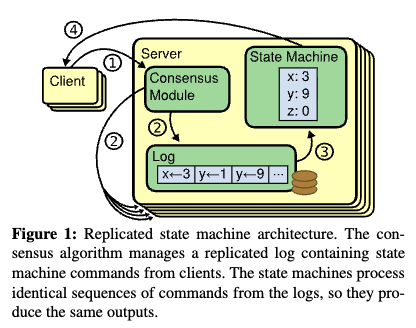
A minimal replicated-state-machine interface looks like this:
```python id=”replicated-state-machine-interface” class ReplicatedStateMachine: def submit(self, command: dict) -> dict: “”” Called by clients.
    The command is first committed through a replicated log.
    Only after commitment is it applied to the local deterministic
    state machine.
    """
    index = consensus.propose(command)
    committed_command = consensus.wait_committed(index)
    return self.apply(committed_command)

def apply(self, command: dict) -> dict:
    """
    Must be deterministic. No random choices, no local wall-clock decisions,
    no non-idempotent external calls inside the state transition.
    """
    raise NotImplementedError ```
The determinism requirement is not optional. If one replica calls random(), reads local time, queries a non-replicated service, or performs a side effect during state-machine execution, replicas can diverge even if the log is identical. The usual implementation rule is: decide nondeterministic values before log append, put them in the command, and make application deterministic.
```python id=”deterministic-command” def create_order_request(user_id: str, cart: dict) -> dict: return { “command_type”: “CreateOrder”, “order_id”: new_uuid(), “created_at_ms”: now_ms(), “user_id”: user_id, “cart”: cart, }
def apply_create_order(state, command): state.orders[command[“order_id”]] = { “user_id”: command[“user_id”], “cart”: command[“cart”], “created_at_ms”: command[“created_at_ms”], }
### Replication is broader than consensus

Consensus is one way to replicate state, but not all replication uses consensus. The right replication method depends on the consistency contract and failure model.

| Pattern                      | Write path                                        | Read path                 | Consistency tendency            | Common use                        |
| ---------------------------- | ------------------------------------------------- | ------------------------- | ------------------------------- | --------------------------------- |
| Asynchronous leader-follower | Leader commits locally, followers catch up later  | Leader or followers       | Eventual or read-after-leader   | Read replicas, analytics replicas |
| Synchronous primary-backup   | Primary waits for backup acknowledgements         | Usually primary           | Stronger, depending on failover | Storage services, metadata        |
| Quorum replication           | Write to $$W$$ of $$N$$, read from $$R$$ of $$N$$ | Quorum read or local read | Tunable                         | Key-value stores                  |
| Chain replication            | Head handles updates, tail handles reads          | Tail                      | Strong per-object consistency   | Storage services                  |
| Consensus log                | Leader or protocol orders commands through quorum | Committed log or leader   | Linearizable writes             | Metadata, locks, control planes   |
| Optimistic multi-master      | Replicas accept local writes and reconcile        | Local replica             | Eventual, conflict-prone        | Mobile, edge, local-first apps    |

[Optimistic Replication](https://pages.cs.wisc.edu/~remzi/Classes/739/Fall2015/Papers/saito-optimistic-05.pdf) by Saito et al. (2005) surveys replication systems that allow short-term divergence to support availability and disconnected work, while [The Dangers of Replication and a Solution](https://db.cs.berkeley.edu/cs286/papers/dangers-sigmod1996.pdf) by Gray et al. (1996) explains why eager replication with transactional consistency can become expensive as update-anywhere replication scales.

The implementation lesson is that “replicated” does not imply “strongly consistent.” A cache, an async replica, a quorum store, a consensus group, and a CRDT are all replicated, but they expose different guarantees.

### Leader-follower replication

Leader-follower replication has one node that accepts writes and one or more followers that copy the leader’s log. The leader serializes writes, appends them to a log, and ships log records to followers. Followers apply records in order.

A simple leader write path:

```python id="leader-follower-basic"
def write_to_leader(command):
    entry = {
        "index": log.next_index(),
        "term": current_term,
        "command": command,
    }

    log.append(entry)
    durable_fsync(log)

    for follower in followers:
        send_async(follower, "AppendLogEntry", entry)

    apply_to_state_machine(entry)
    return {"status": "committed", "index": entry["index"]}
This version is fast but unsafe for automatic failover. The leader returns success after only its own durable write. If the leader crashes before followers receive the entry, a promoted follower may not contain the acknowledged write. This is acceptable only if the durability contract says acknowledged writes can be lost after primary failure, which most systems do not want.
A safer synchronous version waits for enough replicas:
```python id=”leader-follower-synchronous” def write_to_leader(command): entry = { “index”: log.next_index(), “term”: current_term, “command”: command, }
log.append(entry)
durable_fsync(log)

acknowledgements = 1

for follower in followers:
    if send_append_and_wait(follower, entry):
        acknowledgements += 1

if acknowledgements < write_quorum_size():
    raise Unavailable("not enough replicas acknowledged")

mark_committed(entry.index)
apply_to_state_machine(entry)
return {"status": "committed", "index": entry["index"]} ```
This is the shape of many consensus and primary-backup systems, but the correctness depends on the election protocol. Waiting for a majority before acknowledging helps durability, but it does not by itself prevent split brain. The system also needs a rule ensuring that a new leader cannot be elected unless it has enough committed history, or can safely recover that history.
Quorum replication
A quorum is a subset of replicas large enough to overlap with other important subsets. In a system with \(N\) replicas, a write quorum size \(W\), and a read quorum size \(R\), the classic read-write overlap rule is:
\[R + W > N.\]If this holds, every read quorum intersects every write quorum in at least one replica. For majority quorum systems:
\[Q = \left\lfloor \frac{N}{2} \right\rfloor + 1.\]With \(N = 2f + 1\) replicas, a majority quorum has size \(f + 1\), and the system can tolerate \(f\) crash failures for quorum availability:
\[N = 2f + 1 \implies Q = f + 1.\]Examples:
| Replicas \(N\) | Majority quorum \(Q\) | Crash failures tolerated \(f\) |
|---|---|---|
| 1 | 1 | 0 |
| 3 | 2 | 1 |
| 5 | 3 | 2 |
| 7 | 4 | 3 |
A quorum write with versions:
```python id=”quorum-write” def quorum_write(key, value, version): acks = []
for replica in replicas_for(key):
    try:
        replica.put(key, value, version)
        acks.append(replica)
    except ReplicaUnavailable:
        pass

if len(acks) < W:
    raise Unavailable("write quorum not reached")

return {"version": version, "replicas": len(acks)} ```
A quorum read can fetch multiple versions and choose the latest according to a version rule:
```python id=”quorum-read” def quorum_read(key): responses = []
for replica in replicas_for(key):
    try:
        responses.append(replica.get(key))
    except ReplicaUnavailable:
        pass

if len(responses) < R:
    raise Unavailable("read quorum not reached")

latest = max(responses, key=lambda r: r.version)

for response in responses:
    if response.version < latest.version:
        send_async(response.replica, "Repair", latest)

return latest.value ```
This pattern needs careful conflict handling. If the system allows concurrent writes without a single leader, two writes may have incomparable versions. Dynamo-style systems use vector clocks and reconciliation because they choose high availability and allow divergent versions under failures. Dynamo: Amazon’s Highly Available Key-value Store by DeCandia et al. (2007) is the canonical production example of quorum-like replication, sloppy quorums, versioning, hinted handoff, and application-assisted conflict resolution.
Flexible quorums
Majority quorums are simple, but they are not the only safe choice. The deeper requirement is quorum intersection across the protocol steps that need to transfer knowledge. Flexible Paxos: Quorum Intersection Revisited by Howard et al. (2016) shows that Paxos does not require every quorum to intersect every other quorum; the phase-1 quorum for a later proposal must intersect the phase-2 quorums for earlier proposals.
The standard majority rule is:
\[|Q_1| > \frac{N}{2},\quad |Q_2| > \frac{N}{2}.\]Flexible Paxos relaxes this to cross-phase intersection:
\[\forall Q_1 \in \mathcal{Q}_1,\ \forall Q_2 \in \mathcal{Q}_2,\ Q_1 \cap Q_2 \neq \emptyset.\]The practical implication is that quorum geometry can be tuned for deployment goals. A system may use larger leader-election quorums and smaller steady-state replication quorums, or shape quorums around zones and regions. This is advanced because it changes availability and latency tradeoffs, and it is easy to get wrong without formal reasoning.
Chain replication
Chain replication arranges replicas in an ordered chain. Updates enter at the head, flow through intermediate replicas, and complete at the tail. Reads go to the tail. Because the tail has processed all completed updates in order, it can serve strongly consistent reads for the object. Chain Replication for Supporting High Throughput and Availability by van Renesse et al. (2004) presents this design for fail-stop storage servers and argues that strong consistency can coexist with high throughput and availability for large-scale storage services.
The following figure (source) shows the chain replication topology, where update requests enter at the head, query requests are served by the tail, and updates propagate along reliable FIFO links until the tail completes them.
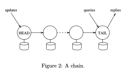
A simplified chain update path:
```python id=”chain-replication-update” def handle_update_at_head(command): result = apply_update(command) forward_to_successor({ “command”: command, “result”: result, })
def handle_update_at_middle(message): apply_replicated_update(message[“command”], message[“result”]) forward_to_successor(message)
def handle_update_at_tail(message): apply_replicated_update(message[“command”], message[“result”]) send_ack_to_client(message[“command”][“request_id”])
A simplified chain read path:

```python id="chain-replication-read"
def handle_query_at_tail(query):
    return read_local_state(query)
The key chain-replication invariant is that if replica \(i\) appears before replica \(j\) in the chain, then \(j\) has a suffix relation to completed work that makes the tail the authority for completed reads. In the original paper, the update propagation invariant tracks how update histories move from head to tail and explains why reads at the tail are strongly consistent.
Chain replication is useful when reads are frequent and can be directed to a tail, and when per-object ordering is enough. It still needs a reliable master or control plane to detect failures, repair chains, and publish the current head and tail. The paper explicitly notes that a real implementation cannot assume an infallible master, and its prototype replicated the master with Paxos.
Primary-backup replication
Primary-backup replication designates one primary to order operations and one or more backups to maintain copies. The primary can reply after local execution, after one backup acknowledgement, after all backup acknowledgements, or after quorum acknowledgement. Each choice changes latency and durability.
| Acknowledgement point | Latency | Failure behavior |
|---|---|---|
| Primary memory only | Lowest | Lost on primary crash |
| Primary durable log | Low | Survives process crash, not host or disk loss |
| One backup durable | Medium | Survives primary loss if backup is promoted safely |
| Majority durable | Higher | Survives minority failure |
| All replicas durable | Highest | Sensitive to slowest replica |
A common write path:
```python id=”primary-backup” def primary_write(command): entry = append_to_local_wal(command) durable_fsync(local_wal)
required = replication_policy.required_acks
acks = 1

for backup in backups:
    if backup.append(entry):
        acks += 1

if acks < required:
    raise Unavailable("replication policy not satisfied")

commit_index = entry.index
apply_until(commit_index)
return {"committed_index": commit_index} ```
Primary-backup becomes difficult during failover. A backup must not become primary if it is missing committed updates. A stale primary must not continue writing after losing authority. The usual tools are terms, epochs, leases, fencing tokens, and consensus-backed membership.
Consensus as ordered agreement
Consensus solves the problem of agreement despite failures. Single-decree consensus chooses one value. Multi-decree consensus chooses a sequence of values, which is how replicated logs are built. The safety properties from Paxos Made Simple by Lamport (2001) are: only a proposed value may be chosen, only a single value is chosen, and a process never learns that a value was chosen unless it actually was chosen.
For a log, this becomes:
\[\text{At most one command can be chosen for log index } i.\]A consensus log gives the application an append API:
```python id=”consensus-log-api” class ConsensusLog: def propose(self, command: dict) -> int: “”” Replicate command and return a committed log index. “”” raise NotImplementedError
def committed_entries_since(self, index: int) -> list[dict]:
    """
    Return committed entries in increasing log-index order.
    """
    raise NotImplementedError ```
The application should not know whether the implementation uses Paxos, Raft, Zab, or Viewstamped Replication. It should only depend on the log contract.
Paxos
Paxos uses proposers, acceptors, and learners. In practice, one process may play several roles. The core idea is that values become chosen when accepted by a quorum, and later proposers must learn enough from earlier acceptors to avoid choosing a conflicting value. Paxos Made Simple by Lamport (2001) is the most accessible canonical paper because it removes the Greek-parliament framing and derives the safety rules from the need to choose one value.
Single-decree Paxos has two broad phases:
| Phase | Proposer action | Acceptor action | Purpose |
|---|---|---|---|
| Prepare | Ask acceptors to promise not to accept lower proposal numbers | Reply with promise and any previously accepted value | Discover prior accepted values |
| Accept | Ask acceptors to accept a value for the proposal number | Accept if no higher promise was made | Choose a value if quorum accepts |
Simplified acceptor state:
```python id=”paxos-acceptor” class Acceptor: def init(self): self.promised_n = None self.accepted_n = None self.accepted_value = None
def prepare(self, n):
    if self.promised_n is None or n > self.promised_n:
        self.promised_n = n
        persist(self.promised_n, self.accepted_n, self.accepted_value)
        return {
            "promise": True,
            "accepted_n": self.accepted_n,
            "accepted_value": self.accepted_value,
        }

    return {"promise": False, "promised_n": self.promised_n}

def accept(self, n, value):
    if self.promised_n is None or n >= self.promised_n:
        self.promised_n = n
        self.accepted_n = n
        self.accepted_value = value
        persist(self.promised_n, self.accepted_n, self.accepted_value)
        return {"accepted": True}

    return {"accepted": False, "promised_n": self.promised_n} ```
The important implementation detail is durability. An acceptor’s promises and accepted values must survive crashes, or a restarted acceptor can violate safety by forgetting a promise. This is why consensus systems depend on write-ahead logs, fsync policy, snapshots, and careful recovery.
Multi-Paxos
Single-decree Paxos chooses one value. A replicated log needs many values, one per index. Multi-Paxos runs repeated Paxos instances, but optimizes the common case by electing a stable leader. Once a leader has completed the prepare phase for a term or ballot, it can append many log entries with accept-style messages, reducing steady-state latency.
The steady-state shape is:
\[\text{client} \rightarrow \text{leader} \rightarrow \text{quorum of acceptors} \rightarrow \text{leader} \rightarrow \text{client}.\]This is why many production consensus systems look leader-based even if their theoretical foundation is Paxos. Google’s The Chubby lock service for loosely-coupled distributed systems by Burrows (2006) describes a coarse-grained lock and low-volume reliable storage service built on distributed consensus; the relevant deployment lesson is that Chubby was used for leader election, metadata, name service, and configuration roots, not high-throughput data-plane storage.
Raft
Raft is a leader-based consensus algorithm designed to be easier to understand and implement than Paxos. It decomposes consensus into leader election, log replication, and safety, and later adds membership changes and log compaction. In Search of an Understandable Consensus Algorithm by Ongaro et al. (2014) states that Raft uses a strong leader, randomized timers for leader election, and joint consensus for membership changes.
A Raft server is always in one of three roles:
| Role | Behavior |
|---|---|
| Follower | Responds to leaders and candidates |
| Candidate | Starts elections after timeout |
| Leader | Accepts client commands and replicates log entries |
The following figure (source) shows Raft’s core safety properties and server-state transitions, including follower, candidate, and leader roles across election terms.
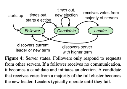
Raft uses monotonically increasing terms:
\[\text{term}_{t+1} > \text{term}_t.\]Each server persists:
| State | Meaning |
|---|---|
currentTerm |
Latest term observed |
votedFor |
Candidate voted for in current term |
log[] |
Sequence of log entries, each with index, term, command |
Each leader also maintains:
| State | Meaning |
|---|---|
nextIndex[follower] |
Next log index to send to that follower |
matchIndex[follower] |
Highest log index known replicated on that follower |
commitIndex |
Highest log index known committed |
A simplified Raft server state:
```python id=”raft-state” class RaftNode: def init(self, node_id, peers): self.node_id = node_id self.peers = peers
    # Persistent state.
    self.current_term = 0
    self.voted_for = None
    self.log = []

    # Volatile state.
    self.commit_index = 0
    self.last_applied = 0

    # Leader-only volatile state.
    self.next_index = {}
    self.match_index = {}

    self.role = "follower" ```
Raft leader election
Followers expect periodic heartbeats from the leader. If a follower receives no valid leader communication before its randomized election timeout, it becomes a candidate, increments its term, votes for itself, and sends RequestVote RPCs. A candidate becomes leader if it receives votes from a majority. Raft’s paper explains that randomized election timers resolve conflicts simply and rapidly, while the majority rule ensures at most one leader can win a term.
The election quorum rule:
\[\text{votes} \geq \left\lfloor \frac{N}{2} \right\rfloor + 1.\]A simplified vote handler:
```python id=”raft-request-vote” def handle_request_vote(self, request): if request.term < self.current_term: return {“term”: self.current_term, “vote_granted”: False}
if request.term > self.current_term:
    self.current_term = request.term
    self.voted_for = None
    self.role = "follower"
    persist_term_and_vote(self.current_term, self.voted_for)

already_voted = self.voted_for is not None and self.voted_for != request.candidate_id
candidate_log_ok = is_candidate_log_at_least_as_up_to_date(
    candidate_last_index=request.last_log_index,
    candidate_last_term=request.last_log_term,
    local_log=self.log,
)

if already_voted or not candidate_log_ok:
    return {"term": self.current_term, "vote_granted": False}

self.voted_for = request.candidate_id
persist_term_and_vote(self.current_term, self.voted_for)

return {"term": self.current_term, "vote_granted": True} ```
The “up-to-date log” check is crucial. It prevents a candidate missing committed entries from becoming leader. In Raft, a candidate’s log is at least as up-to-date if its last log term is greater than the voter’s last log term, or the terms are equal and its last index is at least as large.
```python id=”raft-log-up-to-date” def is_candidate_log_at_least_as_up_to_date( candidate_last_index, candidate_last_term, local_log, ): local_last_index = len(local_log) local_last_term = local_log[-1].term if local_log else 0
if candidate_last_term != local_last_term:
    return candidate_last_term > local_last_term

return candidate_last_index >= local_last_index ```
Raft log replication
The Raft leader appends client commands to its log and sends AppendEntries RPCs to followers. Each RPC includes the previous log index and term so the follower can verify that its log matches the leader’s log prefix. If the check fails, the follower rejects the append, and the leader backs up nextIndex until it finds a matching prefix. The Raft paper calls this the Log Matching Property: if two entries in different logs have the same index and term, then the logs are identical in all preceding entries.
Simplified append handler:
```python id=”raft-append-entries” def handle_append_entries(self, request): if request.term < self.current_term: return {“term”: self.current_term, “success”: False}
self.role = "follower"
self.current_term = request.term

if not log_contains(request.prev_log_index, request.prev_log_term):
    return {"term": self.current_term, "success": False}

delete_conflicting_entries_from(request.prev_log_index + 1)
append_new_entries(request.entries)
persist_log(self.log)

if request.leader_commit > self.commit_index:
    self.commit_index = min(request.leader_commit, last_log_index())
    apply_committed_entries()

return {"term": self.current_term, "success": True} ```
The leader commits an entry once it is stored on a majority and, in Raft’s conservative rule, the entry is from the leader’s current term. Once a current-term entry is committed, earlier entries are committed indirectly through the log-matching property. The Raft paper explicitly notes that Raft does not commit entries from previous terms merely by counting replicas, because such entries can be unsafe in certain histories.
```python id=”raft-commit-rule” def advance_commit_index(self): for index in range(last_log_index(), self.commit_index, -1): replicated = 1
    for peer in self.peers:
        if self.match_index.get(peer, 0) >= index:
            replicated += 1

    entry_is_current_term = self.log[index - 1].term == self.current_term

    if replicated >= majority_size() and entry_is_current_term:
        self.commit_index = index
        apply_committed_entries()
        return ```
Why terms and epochs matter
Terms, epochs, ballots, and views are ways to identify authority. A message from an old leader should not be accepted after a newer term is known. This is what prevents stale leaders from continuing to mutate state after a partition heals.
The basic rule is:
\[\text{accept message} \iff \text{message.term} \geq \text{local.currentTerm}.\]If a node observes a higher term, it steps down:
```python id=”term-step-down” def observe_term(self, remote_term): if remote_term > self.current_term: self.current_term = remote_term self.role = “follower” self.voted_for = None persist_term_and_vote(self.current_term, self.voted_for)
In production, the same concept appears as fencing tokens for leases, generation numbers for controllers, shard ownership epochs, object-store generation preconditions, Kubernetes resource versions, and database compare-and-swap versions.

### Commit index, applied index, and durability

A replicated log has several different positions:

| Position       | Meaning                                        |
| -------------- | ---------------------------------------------- |
| Last log index | Highest entry stored locally                   |
| Commit index   | Highest entry known committed                  |
| Applied index  | Highest entry applied to the state machine     |
| Snapshot index | Highest entry included in a compacted snapshot |

These must not be confused. A follower can store an entry before it is committed. A leader can commit an entry before every follower has it. A state machine should only apply committed entries in order.

```python id="apply-committed-entries"
def apply_committed_entries(self):
    while self.last_applied < self.commit_index:
        self.last_applied += 1
        entry = self.log[self.last_applied - 1]
        result = state_machine.apply(entry.command)
        record_apply_result(entry.index, result)
The write-ahead log must persist entries before the server acknowledges replication. A server that acknowledges an entry and then loses it after crash can break safety. Systems therefore care about fsync grouping, disk latency, write batching, storage corruption, checksums, and replay correctness.
Read paths in consensus systems
Writes clearly require log replication, but reads have several options. The correct read path depends on whether the system promises linearizability.
| Read type | Mechanism | Latency | Risk |
|---|---|---|---|
| Leader local read without check | Read from leader memory | Low | Unsafe if leader is stale |
| Leader lease read | Read if leader lease is valid | Low | Requires clock assumptions and fencing |
| Read index or quorum-confirmed read | Leader confirms it is still leader with quorum | Medium | Safer under partitions |
| Log read | Append a no-op or read command through consensus | Higher | Strong and simple |
| Follower read | Read from follower | Low | Usually stale unless bounded or checked |
| Snapshot read | Read historical version | Low to medium | Requires MVCC and timestamp contract |
A safe but expensive approach is to put reads through the log:
```python id=”linearizable-log-read” def linearizable_read(query): index = consensus.propose({“type”: “ReadBarrier”}) consensus.wait_committed(index) state_machine.apply_until(index) return state_machine.read(query)
A more efficient approach is a read barrier. The leader confirms with a quorum that it is still the current leader, then serves the read after applying all entries committed before that point.

```python id="read-index"
def read_index(query):
    barrier_index = leader.commit_index

    if not confirm_leadership_with_quorum():
        raise NotLeader()

    state_machine.apply_until(barrier_index)
    return state_machine.read(query)
Leases can make reads faster, but only if the deployment can bound clock uncertainty and the protected resource enforces stale-leader rejection. Spanner uses Paxos leader leases, and Spanner: Google’s Globally-Distributed Database by Corbett et al. (2012) describes timed Paxos leader leases and TrueTime-based uncertainty management in a globally replicated database.
Snapshots and log compaction
A consensus log cannot grow forever. Replicas periodically compact old log entries into snapshots. A snapshot captures state up to a specific log index and term. After the snapshot is durable, log entries before that index can be discarded.
The snapshot invariant is:
\[\text{snapshot at index } i \equiv \text{state after applying log entries } 1 \ldots i.\]A snapshot record usually includes:
| Field | Purpose |
|---|---|
last_included_index |
Highest log index represented |
last_included_term |
Term of that log entry |
state_machine_bytes |
Serialized application state |
cluster_configuration |
Membership at snapshot point, if needed |
checksum |
Corruption detection |
Simplified snapshot logic:
```python id=”snapshot-compaction” def maybe_snapshot(self): if log_size_bytes() < SNAPSHOT_THRESHOLD: return
snapshot = {
    "last_included_index": self.last_applied,
    "last_included_term": term_at(self.last_applied),
    "state": state_machine.serialize(),
    "configuration": current_configuration(),
}

write_snapshot_atomically(snapshot)
truncate_log_prefix(up_to_index=self.last_applied) ```
A lagging follower may need an InstallSnapshot RPC instead of ordinary append entries:
```python id=”install-snapshot” def install_snapshot(self, snapshot): if snapshot.last_included_index <= self.snapshot_index: return
write_snapshot_atomically(snapshot)
state_machine.restore(snapshot.state)

self.snapshot_index = snapshot.last_included_index
self.snapshot_term = snapshot.last_included_term
discard_log_entries_through(snapshot.last_included_index) ```
Snapshotting is operationally tricky because snapshots can be large. Production systems throttle snapshot transfer, chunk snapshots, verify checksums, avoid saturating disks, and alert when followers repeatedly fall too far behind.
Membership and reconfiguration
Consensus groups must change membership when nodes are added, removed, replaced, upgraded, or moved across zones. Reconfiguration is dangerous because two different configurations can each believe they have a majority unless the transition is designed to overlap safely.
Raft’s joint consensus approach transitions through a configuration where both old and new majorities are required. Ongaro et al. describe this as joint consensus, where majorities of two different configurations overlap during transitions.
Let \(C_{\text{old}}\) be the old configuration and \(C_{\text{new}}\) the new one. During joint consensus, a log entry must be accepted by majorities of both:
\[\text{commit}*{joint}(e) \iff \text{majority}*{C_{\text{old}}}(e) \land \text{majority}*{C*{\text{new}}}(e).\]A safe reconfiguration sequence:
```python id=”joint-consensus-reconfiguration” def change_membership(new_members): old_members = current_members()
joint_config = {
    "old": old_members,
    "new": new_members,
    "mode": "joint",
}

consensus.propose({
    "type": "ConfigChange",
    "configuration": joint_config,
})

final_config = {
    "members": new_members,
    "mode": "stable",
}

consensus.propose({
    "type": "ConfigChange",
    "configuration": final_config,
}) ```
Many systems add new members as non-voting learners first. A learner receives replicated log entries but does not count toward quorum. Once it catches up, it can be promoted to voting membership. This avoids adding an empty replica to the quorum path and accidentally reducing availability.
```python id=”learner-promotion” def add_member_as_learner(node_id): propose_config_change({“add_learner”: node_id})
while replication_lag(node_id) > MAX_PROMOTION_LAG:
    sleep_with_jitter()

propose_config_change({"promote_to_voter": node_id}) ```
Viewstamped Replication and Zab
Raft is not the only replicated-log protocol. Viewstamped Replication and Zab are important because they show similar leader-based structure with different terminology and system context.
Viewstamped Replication Revisited by Liskov et al. (2012) presents a crash-fault-tolerant replication protocol with views, primaries, backups, normal operation, view changes, recovery, and reconfiguration. Its relevance is that it gives a complete primary-backup consensus-style protocol with explicit handling for client requests, primary failure, replica recovery, and group membership.
Zab: High-performance broadcast for primary-backup systems by Junqueira et al. describes the crash-recovery atomic broadcast protocol used by ZooKeeper. ZooKeeper: Wait-free coordination for Internet-scale systems by Hunt et al. (2010) explains the coordination service built on this approach, including FIFO client ordering and linearizable writes, while serving reads locally for high read throughput.
The practical takeaway is that Paxos, Raft, VR, and Zab differ in mechanics and presentation, but deployed systems usually expose the same shape: a replicated log, epochs or views, one leader or primary in the common case, quorum-based commitment, recovery for lagging replicas, and reconfiguration.
Coordination services
Consensus is expensive enough that many systems centralize it into a coordination service rather than embed it everywhere. Chubby, ZooKeeper, and etcd are examples.
| Service | Core abstraction | Common use |
|---|---|---|
| Chubby | Files, locks, sessions | Coarse-grained locks, leader election, metadata roots |
| ZooKeeper | Hierarchical znodes, watches, sessions | Coordination, configuration, naming, leader election |
| etcd | Replicated key-value store over Raft | Kubernetes state, service metadata, configuration |
The Chubby lock service for loosely-coupled distributed systems by Burrows (2006) emphasizes reliability, availability, and simple semantics over high throughput, and notes that Google systems used it for leader election, metadata, name service, and configuration roots.
ZooKeeper: Wait-free coordination for Internet-scale systems by Hunt et al. (2010) describes a replicated coordination kernel with wait-free reads, FIFO client ordering, and linearizable writes, which is useful because many coordination recipes can be implemented at the client layer.
etcd-io/raft describes etcd’s Raft library as maintaining a replicated state machine through a replicated log, while the etcd FAQ states that etcd uses a leader-based consensus protocol for consistent data replication and log execution.
Leader election with a coordination service
A common deployment pattern is not to make every application implement consensus. Instead, the application uses a coordination service to elect a leader, store a lease, or claim a shard.
A safe leader-election pattern needs fencing:
```python id=”coordination-service-leader-election” def try_become_leader(instance_id): token = coordination_service.increment_and_get(“/service/leader-token”)
acquired = coordination_service.create_ephemeral(
    path="/service/leader",
    value={
        "instance_id": instance_id,
        "fencing_token": token,
    },
)

if not acquired:
    return None

return {"instance_id": instance_id, "fencing_token": token} ```
Every downstream side effect should carry the fencing token:
```python id=”fenced-side-effect” def write_as_leader(fencing_token, update): current = db.get(“resource_owner”)
if fencing_token < current["last_fencing_token"]:
    raise StaleLeader("fencing token is stale")

db.update(
    "resource_owner",
    {
        "last_fencing_token": fencing_token,
        "payload": update,
    },
) ```
The lock or ephemeral node alone is not enough. A process can pause, lose its session, and resume. Fencing ensures that stale leaders are rejected by the resource they are trying to modify.
Split brain
Split brain occurs when two nodes or partitions both believe they are the active authority. It can be caused by network partitions, unsafe failover scripts, stale leases, clock skew, misconfigured load balancers, manual operator intervention, or storage systems that accept writes from an old primary.
A split-brain prevention checklist:
| Risk | Mitigation |
|---|---|
| Old leader continues writing | Terms, epochs, fencing tokens |
| Two nodes acquire lock | Consensus-backed lock service, session semantics |
| Lease holder pauses | Lease TTL plus fencing at resource layer |
| Failover promotes stale replica | Election requires up-to-date log |
| Operator forces primary on both sides | Runbooks with quorum checks and write fences |
| DNS points clients to old primary | Client-side term validation or server-side rejection |
The invariant is:
\[\text{At most one authority may perform writes for epoch } e.\]In code:
```python id=”epoch-write-check” def accept_write(request): if request.epoch != current_epoch: raise StaleEpoch({ “current_epoch”: current_epoch, “request_epoch”: request.epoch, })
apply_write(request) ```
The resource layer must enforce this check. A control plane that knows the correct leader cannot protect a storage node that accepts stale writes.
Geo-replication and consensus placement
Consensus latency depends on quorum placement. If replicas are in one region, quorum round trips are low, but regional failures can take the system down. If replicas span regions, the system can survive regional failures but every strongly consistent write may wait for wide-area latency.
For leader-based quorum replication, steady-state write latency is roughly:
\[L_{\text{write}} \approx L_{\text{client-to-leader}} + \max_{r \in Q} L_{\text{leader-to-replica } r} + L_{\text{fsync}}.\]This is simplified, but it explains why leader placement matters. A leader far from clients adds client-to-leader latency. A quorum spread across continents adds replication latency. A slow disk adds fsync latency.
Spanner combines Paxos groups with time-bounded uncertainty through TrueTime, and uses leader leases for Paxos leadership. Spanner: Google’s Globally-Distributed Database by Corbett et al. (2012) is relevant here because it shows how a global database composes replication, Paxos, leases, MVCC, and clock uncertainty into one externally consistent system.
Advanced consensus variants try to reduce wide-area latency or distribute leader bottlenecks. There Is More Consensus in Egalitarian Parliaments by Moraru et al. (2013) introduces EPaxos, a leaderless Paxos variant that can commit non-conflicting commands with low wide-area latency and balanced load, but at the cost of more protocol complexity.
Replication lag
Replication lag is the distance between a leader’s committed state and a follower’s applied state. It can be measured in bytes, log indexes, seconds, or operations.
\[\text{lag}_{index}(r) = \text{leader.commitIndex} - \text{follower.matchIndex}_r.\] \[\text{lag}*{time}(r) = t*{\text{now}} - t_{\text{last applied entry on follower}}.\]Lag matters because it affects failover safety, read staleness, recovery time, backup freshness, and snapshot transfer.
A lag monitor:
```python id=”replication-lag-monitor” def check_replication_lag(leader): for follower in leader.followers: index_lag = leader.commit_index - leader.match_index.get(follower.id, 0) time_lag_ms = now_ms() - follower.last_apply_time_ms
    metrics.gauge("replication.index_lag", index_lag, tags={"follower": follower.id})
    metrics.gauge("replication.time_lag_ms", time_lag_ms, tags={"follower": follower.id})

    if index_lag > MAX_SAFE_LAG:
        alert("replica lag too high", follower=follower.id, lag=index_lag) ```
Failover systems should not promote a replica solely because it is alive. They should evaluate whether the replica is eligible, sufficiently up to date, in the current configuration, and able to obtain quorum.
Anti-entropy and repair
Not every replicated system uses consensus for every update. Eventually consistent stores often use anti-entropy repair: replicas compare summaries of their data and exchange missing or stale records. This can use Merkle trees, version vectors, per-partition hashes, tombstone propagation, or background read repair.
A simple repair loop:
```python id=”anti-entropy-repair” def repair_partition(partition_id, replicas): digests = { replica.id: replica.compute_digest(partition_id) for replica in replicas }
if all_equal(digests.values()):
    return

differences = compare_digests(digests)

for key in differences.keys:
    versions = [replica.get(key) for replica in replicas]
    resolved = resolve_versions(versions)

    for replica in replicas:
        if replica.get(key).version < resolved.version:
            replica.put(key, resolved.value, resolved.version) ```
Anti-entropy is for convergence, not immediate safety. It works when the application can tolerate temporary divergence or has a conflict-resolution model. It is not appropriate for leader election, money movement, unique username allocation, or anything else that requires a single immediate decision.
Replication and external side effects
A replicated state machine should not directly perform external non-idempotent side effects while replaying commands. If it sends an email, charges a credit card, or calls another service during log application, a replay, snapshot restore, or leader change can duplicate the effect.
Bad pattern:
```python id=”side-effect-inside-state-machine-bad” def apply(command): if command[“type”] == “ChargeCard”: payment_api.charge(command[“card”], command[“amount”]) state.payments[command[“payment_id”]] = “charged”
Safer pattern: commit intent in the replicated log, then have an external worker perform the side effect with an idempotency key.

```python id="side-effect-outbox-safe"
def apply(command):
    if command["type"] == "RequestCharge":
        state.payments[command["payment_id"]] = "pending"
        state.outbox.append({
            "message_id": command["payment_id"],
            "type": "ChargeCard",
            "idempotency_key": command["payment_id"],
            "amount": command["amount"],
        })

def payment_worker():
    for message in read_outbox():
        payment_api.charge(
            amount=message["amount"],
            idempotency_key=message["idempotency_key"],
        )
        mark_outbox_sent(message["message_id"])
The log decides durable intent. The side-effect system uses idempotency to make retries safe.
Consensus performance knobs
Consensus performance depends on batching, pipelining, disk writes, network latency, serialization cost, snapshotting, and follower lag.
| Knob | Benefit | Risk |
|---|---|---|
| Batch multiple commands per append | Higher throughput | Higher per-command latency |
| Pipeline replication | Better link utilization | More complex flow control |
| Group fsyncs | Lower disk overhead | Larger loss window if misconfigured |
| Use leader leases for reads | Lower read latency | Clock and fencing complexity |
| Use snapshots | Bounded log size | Expensive transfer and restore |
| Add learners before voters | Safer scaling | Longer reconfiguration process |
| Place quorum in one region | Low latency | Regional failure risk |
| Spread quorum across regions | Regional resilience | Higher write latency |
A batched append loop:
```python id=”batched-consensus-append” def leader_replication_loop(): while is_leader(): batch = pending_commands.take_batch(max_items=256, max_wait_ms=5)
    if not batch:
        send_heartbeat()
        continue

    entries = []
    for command in batch:
        entries.append(log.append_uncommitted(command))

    durable_fsync(log)

    replicate_batch_to_followers(entries)
    advance_commit_index() ```
Batching improves throughput because fixed costs are amortized:
\[\text{cost per command} \approx \frac{C_{\text{network}} + C_{\text{fsync}}}{B} + C_{\text{apply}},\]where \(B\) is batch size. The tradeoff is queueing latency: commands wait for the batch to fill or the batch timer to expire.
Consensus availability
Consensus availability requires a quorum. With majority quorums, a group of \(N = 2f + 1\) replicas can tolerate \(f\) unavailable replicas. If more than \(f\) replicas are unavailable or partitioned away from the leader, the group should stop accepting writes.
For a five-node group:
\[N = 5,\quad Q = 3,\quad f = 2.\]If two nodes fail, the remaining three can still make progress. If three nodes fail, the remaining two cannot safely decide new log entries.
Availability is not only a node count. Correlated failures matter. Five replicas in the same rack do not protect against rack failure. Five replicas running the same bad binary do not protect against a deterministic crash bug. Five replicas sharing one control plane do not protect against control-plane misconfiguration.
Production placement should think in failure domains:
| Failure domain | Placement rule |
|---|---|
| Process | Multiple processes |
| Host | Multiple hosts |
| Rack | Spread across racks |
| Zone | Spread across zones if zone failure is in scope |
| Region | Spread across regions only if latency budget allows |
| Software version | Stagger rollouts |
| Operator action | Use automation, policy, and blast-radius limits |
Consensus and deployment systems
Consensus is used heavily in deployment infrastructure, but mostly for metadata and coordination rather than high-volume data-plane work. Kubernetes stores cluster state in etcd, and etcd uses Raft to replicate that state. The etcd Raft library describes Raft as maintaining a replicated state machine through a replicated log, and the etcd FAQ describes leader election, heartbeats, and follower-triggered elections when heartbeats are not received.
A deployment control plane typically uses consensus for:
| State | Why consensus helps |
|---|---|
| Desired cluster state | Controllers need one authoritative view |
| Lease objects | Leaders and controllers need safe ownership |
| Configuration | Rollouts need durable, ordered updates |
| Service discovery metadata | Clients need coherent endpoint sets |
| Locks and elections | Avoid duplicated critical work |
| API object versions | Prevent lost updates and stale writes |
It should avoid putting high-cardinality, high-frequency telemetry or data-plane traffic directly into the consensus store. Consensus-backed stores are usually optimized for small, critical metadata, not for unbounded event streams or large blobs.
Implementation checklist for a consensus-backed service
A production consensus-backed service should specify and test:
- Persistent state: Terms, votes, and log entries are fsynced before acknowledgements.
- Deterministic application: State-machine commands do not depend on local wall-clock time, random choices, or external side effects.
- Leader stepdown: Any higher term forces a leader or candidate to become follower.
- Election restriction: A candidate missing committed history cannot win.
- Commit rule: Entries are applied only after the protocol’s commit condition is met.
- Read safety: Linearizable reads use a log barrier, quorum-confirmed read index, or safe lease.
- Snapshot correctness: Snapshot state exactly matches applied log prefix.
- Follower catch-up: Lagging replicas can receive log entries or snapshots without blocking the leader forever.
- Reconfiguration: Membership changes preserve quorum overlap, preferably through joint consensus or equivalent.
- Learner flow: New replicas catch up as learners before becoming voters.
- Fencing: External resources reject stale leaders using epochs or fencing tokens.
- Backpressure: Slow followers, full disks, and large snapshots do not exhaust memory.
- Observability: Metrics expose term changes, leader changes, commit index, applied index, fsync latency, proposal latency, quorum latency, and replication lag.
- Disaster recovery: Backups, snapshots, and restore procedures are tested, not merely documented.
Common replication and consensus failure modes
| Failure mode | Cause | Fix |
|---|---|---|
| Lost acknowledged write | Leader replied before durable quorum | Ack only after required replication and fsync |
| Split brain | Unsafe failover or stale lease | Terms, quorums, fencing, safe runbooks |
| Stale leader writes | Paused process resumes after losing authority | Resource-level fencing token |
| Election storm | Timeouts too low or network unstable | Randomized timeouts, pre-vote, better health isolation |
| Slow quorum | One required replica is slow | Majority quorum, follower isolation, placement review |
| Log grows forever | Snapshotting absent or broken | Periodic snapshots and compaction |
| Snapshot overload | Large snapshot transfer saturates resources | Chunking, throttling, rate limits |
| Reconfiguration outage | Added empty voter directly | Add learner, catch up, then promote |
| Stale follower reads | Reads served from lagging replica | Read index, leader reads, bounded staleness contract |
| Duplicate side effects | Replayed commands call external APIs | Outbox and idempotency keys |
| Correlated replica failure | Same zone, same binary, same dependency | Failure-domain-aware placement and staged rollout |
| Consensus store overload | High-volume data sent to metadata store | Move events/blobs to logs or object storage |
Design guidance
Use consensus when the system needs one authoritative decision: leader election, metadata updates, shard ownership, configuration, locks, schema changes, durable workflow state, or linearizable small records. Avoid consensus when the workload can tolerate stale reads, eventual convergence, per-key ordering, append-only event processing, or local conflict resolution.
A practical rule:
\[\text{Use consensus for control-plane truth; use partitioned logs, storage, and caches for data-plane scale.}\]This is why systems such as Kubernetes rely on etcd for cluster state but do not store container logs, metrics, traces, or application data in etcd. It is also why large distributed databases split data into many independently replicated shards: each shard or range can have its own replication group, leader, log, and placement policy.
Replication gives redundancy. Consensus gives agreement. The art of deployed distributed systems is deciding exactly where agreement is worth its latency and availability cost, then making every boundary around that agreement explicit: terms, quorums, logs, snapshots, read contracts, reconfiguration, fencing, and recovery.
Consistency Models
Why consistency models matter
A consistency model is the contract that tells clients what values they are allowed to observe when operations overlap, replicas lag, transactions interleave, clocks differ, or failures occur. A database, cache, queue, filesystem, object store, coordination service, or replicated log can all be “correct” only relative to a stated model. Consistency Models explains consistency as a set of legal histories, and Linearizability: A Correctness Condition for Concurrent Objects by Herlihy et al. (1990) is the classic paper defining one of the strongest and most useful object-level consistency models.
The same system can expose multiple consistency models. For example, a control-plane key-value store may provide linearizable writes for metadata, stale reads for dashboards, watch streams for controllers, and eventually consistent telemetry for metrics. A distributed SQL database may provide strict serializable transactions for user-facing writes, historical snapshot reads for analytics, and follower reads with bounded staleness for low-latency dashboards. The practical design mistake is to say “the system is consistent” without specifying which operations, which objects, which replicas, which failure modes, and which client observations are covered. Consistency is useful because it separates consistency models from marketing labels and frames them as safety properties over histories.
Histories, operations, and legal executions
A history is a record of operation invocations and responses. For a key-value store, a history might include write(x, 1), read(x) -> 1, write(x, 2), and read(x) -> 2. For a transactional database, each operation might be a transaction containing several reads and writes. A consistency model defines which histories are legal.
A simplified operation record:
```python id=”history-operation” from dataclasses import dataclass from typing import Any
@dataclass(frozen=True) class Operation: process_id: str op_id: str kind: str key: str value: Any | None invoke_time: int response_time: int | None result: Any | None
A consistency checker asks whether there exists an ordering or execution that explains the observed operations:

```python id="consistency-checker-shape"
def is_legal(history: list[Operation], model: str) -> bool:
    candidate_orders = generate_candidate_orders(history, model)

    for order in candidate_orders:
        if respects_model_constraints(order, history, model):
            if satisfies_object_or_transaction_spec(order):
                return True

    return False
The important point is that consistency is not about whether one particular server behaved locally. It is about whether the complete observed history could have happened under the model’s rules. Jepsen is important operationally because it records histories under faults and checks whether real systems satisfy claimed models.
The two axes: object consistency and transactional isolation
Consistency vocabulary can be confusing because two different families of guarantees are often discussed together.
| Family | Unit of reasoning | Examples |
|---|---|---|
| Object consistency | Operations on one object, register, queue, lock, or key | Linearizability, sequential consistency, causal consistency, eventual consistency |
| Transactional isolation | Transactions over multiple objects | Serializability, strict serializability, snapshot isolation, read committed |
Object consistency asks what one object or service can return. Transactional isolation asks how groups of reads and writes interleave. A single-key linearizable register and a multi-key serializable database solve related but different problems. A Critique of ANSI SQL Isolation Levels by Berenson et al. (1995) is useful because it shows that transaction isolation needs precise phenomena beyond informal SQL labels, while Weak Consistency: A Generalized Theory and Optimistic Implementations for Distributed Transactions by Adya (1999) gives implementation-independent definitions for isolation levels and transactional phenomena.
A hierarchy of common consistency models
Consistency models form a partial order. Stronger models rule out more histories and are easier for clients to reason about, but they usually require more coordination, higher latency, or lower availability during partitions. Weaker models permit more histories and are easier to deploy across regions or offline clients, but they push more correctness work into application logic.
The following figure (source) shows an implication hierarchy of consistency models, where stronger models imply weaker ones and weaker models permit more observable histories.
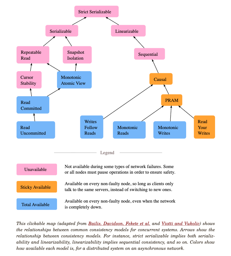
A simplified hierarchy is:
| Model | Core idea | Typical coordination cost |
|---|---|---|
| Strict serializability | Transactions appear in a serial order that respects real time | Very high for distributed writes |
| Linearizability | Each object operation appears instantaneous between invocation and response | High for replicated objects |
| Serializability | Transactions appear equivalent to some serial order | High, but can be optimized |
| Sequential consistency | Operations appear in some process-order-respecting total order | High under partition |
| Causal consistency | Causally related operations are observed in causal order | Medium metadata cost |
| Read-your-writes | A client sees its own prior writes | Low to medium |
| Monotonic reads | A client does not go backward in observed versions | Low to medium |
| Eventual consistency | Replicas converge if updates stop | Low coordination cost |
Jepsen’s model page states, for single-object models, that strict serializable implies linearizable, linearizable implies sequential, sequential implies causal, and causal implies several session guarantees such as read-your-writes and monotonic reads.
Linearizability
Linearizability is one of the strongest and most useful consistency models for replicated objects. An operation appears to take effect atomically at some point between its invocation and response. That point is called the linearization point. If operation A completes before operation B begins, then A must appear before B in the linearized order. Linearizability: A Correctness Condition for Concurrent Objects by Herlihy et al. (1990) defines linearizability and shows why it supports local reasoning about concurrent objects.
The real-time rule is:
\[\text{if } response(A) < invocation(B),\ \text{then } A <_{\text{linearized}} B.\]A linearizable register example:
```text id=”linearizable-history” time → Client 1: write(x = 1) ───────── ok Client 2: read(x) ─── 1
This history is linearizable because the read can be ordered after the write. This one is not linearizable if the write completed before the read began:

```text id="nonlinearizable-history"
time →
Client 1: write(x = 1) ── ok
Client 2:                    read(x) ── 0
Linearizability is usually implemented with a single leader, a consensus log, a quorum protocol, or a storage engine with compare-and-swap over a strongly consistent metadata layer. A safe linearizable read must prove it is reading from an authority that has not been superseded.
```python id=”linearizable-read-index” def linearizable_get(key): if not leader.confirm_still_leader_with_quorum(): raise NotLeader()
leader.apply_until(leader.commit_index)
return state_machine.get(key) ```
The cost is coordination. During a partition, a replica that cannot contact quorum should not accept linearizable writes, and may not be able to serve linearizable reads. This is the same operational tradeoff formalized by CAP-style results for replicated read-write objects. Brewer’s Conjecture and the Feasibility of Consistent, Available, Partition-Tolerant Web Services by Gilbert et al. (2002) formalizes the consistency-availability partition tradeoff, while Herlihy and Wing define the object-level correctness condition itself.
Strict serializability
Strict serializability is the transactional analogue of linearizability. Transactions appear to execute one at a time, and that serial order respects real-time order. If transaction T1 commits before transaction T2 starts, T1 must appear before T2. Strict serializability is often what application developers intuitively mean by “transactions behave correctly,” especially for financial ledgers, inventory, unique constraints, permissions, and metadata changes.
The condition can be stated as:
\[\text{strict serializability} = \text{serializability} + \text{real-time order}.\]A strict serializable system must rule out histories where a later transaction misses a previously committed transaction. Spanner: Google’s Globally-Distributed Database by Corbett et al. (2012) is the canonical deployed example of globally distributed transactions with external consistency, using Paxos replication, MVCC, and TrueTime clock uncertainty. Google Cloud’s Spanner: TrueTime and external consistency explains the operational contract: TrueTime exposes bounded clock uncertainty that Spanner uses for monotonic timestamp assignment across servers.
A simplified commit-wait shape:
```python id=”commit-wait-shape” def commit_transaction(txn): commit_ts = truetime.now_latest()
write_intents_with_timestamp(txn.writes, commit_ts)
replicate_commit_record(txn.id, commit_ts)

# Wait until every future transaction's earliest possible timestamp
# is greater than this commit timestamp.
while truetime.now_earliest() <= commit_ts:
    sleep_shortly()

mark_committed(txn.id)
return {"commit_timestamp": commit_ts} ```
The code is only a sketch. The implementation difficulty is that timestamp assignment, replication, two-phase commit, lock management, and clock uncertainty must be composed without violating real-time order.
Serializability
Serializability says that concurrent transactions are equivalent to some serial execution. Unlike strict serializability, serializability does not necessarily require that the serial order respect wall-clock real-time order. This distinction matters when a system can reorder overlapping transactions safely, but it can surprise clients if a transaction appears to ignore an earlier completed transaction.
A transaction history is serializable if there exists a serial order:
\[T_{\pi(1)}, T_{\pi(2)}, \ldots, T_{\pi(n)}\]such that the observed reads and final writes match that serial execution.
A simple serializable transfer invariant:
```python id=”serializable-transfer” def transfer(tx, from_account, to_account, amount): from_balance = tx.read(from_account) to_balance = tx.read(to_account)
if from_balance < amount:
    raise InsufficientFunds()

tx.write(from_account, from_balance - amount)
tx.write(to_account, to_balance + amount) ```
Under serializability, concurrent transfers must behave as if they happened one at a time. Without serializability, two transfers can both read the same starting balance and overspend.
Serializability can be implemented with strict two-phase locking, optimistic concurrency control with validation, deterministic transaction ordering, or serializable snapshot isolation. Calvin: Fast Distributed Transactions for Partitioned Database Systems by Thomson et al. (2012) is relevant because it uses deterministic ordering to reduce distributed transaction coordination, while Serializable Snapshot Isolation in PostgreSQL by Ports et al. (2012) describes a production implementation of Serializable Snapshot Isolation.
Sequential consistency
Sequential consistency says that operations appear in some total order that respects the order of operations issued by each process, but not necessarily real-time order across processes. Consistency Models describes sequential consistency as requiring a total order consistent with each process’s program order, and notes that sequential consistency is weaker than linearizability because it does not require real-time ordering across processes.
The condition is:
\[\forall p,\ \text{program order of process } p \text{ is preserved in the global order}.\]Sequential consistency allows some histories linearizability rejects. If client 1 writes x = 1, receives success, and then client 2 reads x = 0, the history may still be sequentially consistent if client 2’s read is placed before client 1’s write in the global order. It is not linearizable if the write completed before the read began.
This model is sometimes useful for systems that need per-client ordering but do not want to pay for real-time global ordering. In practice, many distributed storage APIs expose more specific session guarantees rather than plain sequential consistency because the latter is still expensive and not always intuitive for users.
Causal consistency
Causal consistency preserves happened-before relationships. If operation A causally influences operation B, then every client that sees B must also see A. If two writes are concurrent, replicas may observe them in different orders unless a conflict-resolution rule orders or merges them.
Causality is usually modeled using Lamport’s happened-before relation:
\[A \rightarrow B.\]Causal consistency requires:
\[A \rightarrow B \implies \text{any replica that observes } B \text{ must also observe } A.\]A practical example:
```text id=”causal-example” User A: post(“I got the job”) User B: reads post, then comments(“Congrats!”) User C: sees comment
Under causal consistency, user C should not see “Congrats!” without also seeing the original post, because the comment causally depends on the post. Causal consistency is usually implemented with dependency metadata, vector clocks, version vectors, causal broadcast, or session tokens. [Session Guarantees for Weakly Consistent Replicated Data](https://www.cs.cornell.edu/courses/cs734/2000FA/cached%20papers/SessionGuaranteesPDIS_1.html) by Terry et al. (1994) is important because it turns weak replicated storage into a more usable client experience through session-level guarantees such as read-your-writes, monotonic reads, writes-follow-reads, and monotonic writes.

A dependency-carrying write:

```python id="causal-write"
def write_comment(session, post_id, text):
    dependencies = session.observed_versions.copy()

    event = {
        "type": "CommentCreated",
        "post_id": post_id,
        "text": text,
        "dependencies": dependencies,
        "version": new_version(),
    }

    store.write(event)
    session.observe(event["version"])
A replica should not expose the comment until its dependencies are present:
```python id=”causal-visibility” def is_visible(event, replica_versions): for key, required_version in event[“dependencies”].items(): if replica_versions.get(key, 0) < required_version: return False return True
The cost of causal consistency is metadata and dependency tracking. The benefit is that it avoids many user-visible anomalies without requiring every operation to coordinate through a global leader.

### Session guarantees

Session guarantees are weaker than global consistency models but very useful for product behavior. They define what one client session can observe, even when requests are routed to different replicas. Terry et al. proposed four main guarantees: read-your-writes, monotonic reads, writes-follow-reads, and monotonic writes. The purpose is to give users a coherent view of their own actions even when the underlying store is weakly consistent.

| Guarantee           | User-facing meaning                                                 | Implementation pattern                      |
| ------------------- | ------------------------------------------------------------------- | ------------------------------------------- |
| Read-your-writes    | After I update my profile, I see my update                          | Sticky routing, session token, primary read |
| Monotonic reads     | I do not see version 5 and then version 3                           | Session version floor                       |
| Monotonic writes    | My writes are applied in the order I issued them                    | Per-session sequence numbers                |
| Writes-follow-reads | If I write after reading something, my write depends on what I read | Dependency metadata                         |

A session token can carry the minimum version the client must observe:

```python id="session-token"
@dataclass
class SessionToken:
    observed_versions: dict[str, int]

def read_with_session(session: SessionToken, key: str):
    required = session.observed_versions.get(key, 0)

    replica = choose_replica_with_version_at_least(key, required)
    value, version = replica.get(key)

    session.observed_versions[key] = max(required, version)
    return value
If no replica is caught up enough, the system can wait, route to the leader, return a retryable error, or explicitly serve stale data depending on the API contract. The worst option is silently returning older data after the user has already observed newer data.
Eventual consistency
Eventual consistency says that if no new updates are made to an object, replicas eventually converge to the same value. This is a liveness-style convergence promise, not a guarantee that every intermediate read is intuitive. Eventually Consistent by Vogels (2009) explains the consistency-availability tradeoffs behind large-scale replicated systems and discusses client-side consistency variants such as read-your-writes and monotonic reads.
A convergence condition can be written as:
\[\text{if updates stop at time } t,\ \exists t' > t\ \text{such that all non-faulty replicas agree after } t'.\]The implementation usually needs three pieces:
| Mechanism | Purpose |
|---|---|
| Propagation | Spread updates to replicas |
| Versioning | Detect stale, concurrent, or superseded values |
| Resolution | Choose or merge conflicting versions |
A last-writer-wins register is simple but can lose updates:
```python id=”last-writer-wins” def merge_lww(a, b): if a.timestamp > b.timestamp: return a if b.timestamp > a.timestamp: return b return max(a, b, key=lambda item: item.replica_id)
The danger is that concurrent writes are forced into one arbitrary winner. This is fine for ephemeral cache values, bad for shopping carts, collaborative documents, counters, permissions, and financial state. Dynamo’s design exposes divergent versions to application logic because Amazon’s shopping-cart semantics preferred preserving concurrent additions over silently discarding them. [Dynamo: Amazon’s Highly Available Key-value Store](https://www.allthingsdistributed.com/files/amazon-dynamo-sosp2007.pdf) by DeCandia et al. (2007) is the canonical example of application-aware reconciliation in a highly available key-value store.

### Strong eventual consistency and CRDTs

Strong eventual consistency means that replicas that have received the same updates have the same state, even if the updates arrived in different orders. CRDTs achieve this by designing data types whose merge or operations are mathematically safe under concurrency. [Conflict-free Replicated Data Types](https://arxiv.org/abs/1805.06358) by Preguiça et al. (2018) explains that CRDT replicas can be modified independently and deterministically converge when they have received the same set of updates.

For state-based CRDTs, the merge function is usually a join over a semilattice. It should be commutative, associative, and idempotent:

$$
merge(a, b) = merge(b, a)
$$

$$
merge(a, merge(b, c)) = merge(merge(a, b), c)
$$

$$
merge(a, a) = a
$$

A grow-only counter:

```python id="g-counter"
class GCounter:
    def __init__(self, replica_id, replicas):
        self.replica_id = replica_id
        self.counts = {replica: 0 for replica in replicas}

    def increment(self, amount=1):
        self.counts[self.replica_id] += amount

    def value(self):
        return sum(self.counts.values())

    def merge(self, other):
        for replica, count in other.counts.items():
            self.counts[replica] = max(self.counts.get(replica, 0), count)
This counter converges because each replica’s component only increases and merge takes component-wise maximum. CRDTs are excellent for counters, sets, maps, collaborative editing metadata, presence, local-first applications, and offline-capable systems. They are less natural for invariants that require global exclusion, such as “seat count must never go below zero,” “username must be globally unique,” or “only one leader may exist.”
Quorum consistency and tunable reads
Quorum systems expose consistency through read and write quorum sizes. With replicas, read quorum size, and write quorum size, a common overlap rule is:
\[R + W > N.\]This gives read-write quorum intersection, but it does not automatically give linearizability. The system also needs versioning, conflict resolution, failure handling, and a rule for concurrent writes. Vogels’s Eventually Consistent discusses the quorum configuration intuition around read and write sets, while Dynamo shows how quorum-like settings combine with vector clocks and reconciliation in production.
A tunable quorum example:
```python id=”tunable-quorum” def put(key, value, write_quorum): version = next_version(key)
acknowledgements = []
for replica in replicas_for(key):
    if replica.put(key, value, version):
        acknowledgements.append(replica)

if len(acknowledgements) < write_quorum:
    raise Unavailable()

return version
def get(key, read_quorum): responses = [] for replica in replicas_for(key): response = replica.get(key) if response is not None: responses.append(response)
if len(responses) < read_quorum:
    raise Unavailable()

return resolve(responses) ```
Tunable consistency is useful because not every operation needs the same guarantee. A profile image read may tolerate staleness. A password change should not. A product count may tolerate bounded staleness for browsing but not for checkout.
Bounded staleness
Bounded staleness guarantees that reads are stale by at most some version distance or time interval. This sits between linearizable reads and arbitrary stale reads. It is useful for follower reads, dashboards, search indexes, analytics projections, and geo-replicated read replicas.
Version-bounded staleness:
\[\text{leader_version} - \text{replica_version} \leq k.\]Time-bounded staleness:
\[t_{\text{now}} - t_{\text{replica_applied}} \leq \Delta.\]A follower-read guard:
```python id=”bounded-staleness-read” def bounded_stale_read(replica, key, max_staleness_ms): lag_ms = now_ms() - replica.last_applied_time_ms
if lag_ms > max_staleness_ms:
    raise TooStale({
        "lag_ms": lag_ms,
        "max_staleness_ms": max_staleness_ms,
    })

return replica.get(key) ```
The subtle point is how the system measures last_applied_time_ms. If it uses wall-clock timestamps from different machines, clock skew matters. If it uses log positions, clients need a way to compare the replica’s applied position to a known leader or transaction position.
Snapshot isolation
Snapshot isolation gives each transaction a consistent snapshot of committed data as of its start timestamp, and commits only if write-write conflicts are absent. It is popular because reads do not block writes and writes do not block reads. However, ordinary snapshot isolation is not serializable because it can allow write skew. A Critique of ANSI SQL Isolation Levels by Berenson et al. (1995) introduced snapshot isolation as an important multiversion isolation type, and Serializable Snapshot Isolation in PostgreSQL by Ports et al. (2012) explains how PostgreSQL added serializable behavior on top of snapshot isolation using SSI.
Snapshot read rule:
\[read_T(x) = \text{latest committed version of } x \text{ with } commit_ts \leq start_ts(T).\]Commit rule for ordinary snapshot isolation:
\[\text{commit allowed if no concurrent committed transaction wrote the same item}.\]MVCC version lookup:
```python id=”mvcc-read” def mvcc_read(key, snapshot_ts): versions = storage.get_versions(key)
visible = [
    version for version in versions
    if version.commit_ts <= snapshot_ts and not version.deleted
]

if not visible:
    return None

return max(visible, key=lambda version: version.commit_ts).value ```
Write skew example:
```text id=”write-skew” Invariant: at least one doctor must be on call.
T1 reads: Alice on call = true, Bob on call = true T2 reads: Alice on call = true, Bob on call = true
T1 writes: Alice on call = false T2 writes: Bob on call = false
Both transactions write different rows, so ordinary snapshot isolation may allow both. Final state violates the invariant.
The implementation fix is serializable isolation, explicit locking of the predicate, materialized constraint rows, or application-level compare-and-swap over the invariant.

### Isolation levels and anomalies

Isolation levels are best understood by the anomalies they permit or forbid. ANSI SQL labels alone have historically been ambiguous, which is why Berenson et al. and Adya’s thesis are widely cited for formalizing the problem. Jepsen’s [Phenomena](https://jepsen.io/consistency/phenomena) page summarizes Adya-style phenomena such as aborted reads, intermediate reads, cyclic information flow, and anti-dependency cycles.

| Anomaly             | What happens                                                          | Example risk                     |
| ------------------- | --------------------------------------------------------------------- | -------------------------------- |
| Dirty read          | A transaction reads another transaction’s uncommitted write           | Observing data that later aborts |
| Non-repeatable read | A transaction reads the same item twice and sees different values     | Inconsistent decisions           |
| Phantom             | Re-running a predicate query returns different matching rows          | Broken range constraints         |
| Lost update         | Two transactions read the same value and overwrite each other         | Counters, balances, inventory    |
| Read skew           | A transaction observes inconsistent versions of related data          | Broken reports                   |
| Write skew          | Two transactions write disjoint items after reading overlapping state | Broken cross-row invariants      |
| Cyclic dependency   | Transactions form a dependency cycle                                  | Non-serializable execution       |

A lost update pattern:

```python id="lost-update"
# Initial balance = 100

def withdraw_without_guard(account_id, amount):
    balance = db.read(account_id)
    db.write(account_id, balance - amount)
If two transactions both read 100 and both write 90, one withdrawal is lost. A safer pattern uses compare-and-swap:
```python id=”cas-update” def withdraw_with_cas(account_id, amount): while True: account = db.read(account_id)
    if account.balance < amount:
        raise InsufficientFunds()

    updated = account.with_balance(account.balance - amount)

    if db.compare_and_swap(
        key=account_id,
        expected_version=account.version,
        new_value=updated,
    ):
        return updated ```
Compare-and-swap protects one object. Multi-object invariants require transactional isolation or explicit invariant design.
Read committed, repeatable read, and serializable in practice
Real databases differ in how they implement isolation labels, so application code should rely on documented behavior rather than name alone. In broad terms:
| Level | Typical guarantee | Common remaining risk |
|---|---|---|
| Read committed | Reads only committed data | Non-repeatable reads, lost updates unless guarded |
| Repeatable read | Repeated reads of the same row are stable | Predicate anomalies depending on implementation |
| Snapshot isolation | Reads from a consistent snapshot, write-write conflicts detected | Write skew |
| Serializable | Equivalent to serial execution | Abort or blocking under conflicts |
| Strict serializable | Serializable and real-time ordered | Higher distributed coordination cost |
A safe transactional API should make retries part of the contract because serializable systems often abort transactions to preserve correctness.
```python id=”serializable-retry-loop” def run_serializable(work, max_attempts=5): for attempt in range(max_attempts): tx = db.begin(isolation=”serializable”) try: result = work(tx) tx.commit() return result except SerializationFailure: tx.rollback() sleep_with_jitter(attempt)
raise TooMuchContention() ```
This is not an error case in the ordinary sense. It is how optimistic serializable systems preserve correctness under concurrency. Application code must be structured so the transaction body can safely run again.
Consistency and constraints
Consistency models should be chosen by invariant. An invariant is a condition that must remain true over time.
Examples:
| Invariant | Required design pressure |
|---|---|
| Username is globally unique | Linearizable uniqueness check or partitioned authority |
| Bank balance never goes negative | Serializable transaction or escrow-style invariant management |
| Shopping cart preserves all concurrent adds | Mergeable conflict resolution |
| User sees their own profile update | Read-your-writes |
| Search results may lag by 30 seconds | Bounded staleness |
| Metrics eventually converge | Eventual consistency |
| Only one scheduler owns a shard | Consensus, lease, and fencing |
A uniqueness constraint under weak consistency can fail if two replicas accept the same username concurrently. A safe implementation routes all claims for the username to one authority or uses a strongly consistent constraint table.
```python id=”unique-constraint-authority” def claim_username(user_id, username): shard = shard_for_username(username)
return shard.run_linearizable_transaction(
    lambda tx: claim_if_absent(tx, user_id, username)
)
def claim_if_absent(tx, user_id, username): if tx.exists((“username”, username)): raise UsernameTaken()
tx.put(("username", username), {"user_id": user_id}) ```
The more general rule is that invariants involving non-commutative choices usually require coordination. Invariants over monotonic facts can often avoid coordination. Keeping CALM: When Distributed Consistency is Easy by Hellerstein et al. (2019) explains the CALM theorem, which connects coordination-free consistency to logical monotonicity.
Choosing consistency per operation
Many production systems expose multiple consistency levels because no single model is optimal for every operation.
| Operation | Suggested model | Why |
|---|---|---|
| Create account | Linearizable or strict serializable | Avoid duplicate identity or partial creation |
| Change password | Linearizable write, read-your-writes for verification | Security-sensitive |
| View profile | Read-your-writes or bounded stale | User should see own changes, others can lag |
| Browse catalog | Bounded stale or eventual | Low correctness risk |
| Checkout inventory decrement | Serializable or escrow | Prevent oversell |
| Add item to cart | Causal or mergeable eventual | Preserve concurrent additions |
| Emit analytics event | At-least-once eventual | Throughput matters more than immediate consistency |
| Acquire shard lease | Linearizable with fencing | Avoid split brain |
| Query dashboard | Bounded stale snapshot | Stable, cheap reads |
A good API should make the model visible:
```python id=”consistency-aware-api” profile = users.get_profile( user_id, consistency=”read_your_writes”, session_token=session.token, )
inventory = stock.reserve( sku, quantity=1, consistency=”serializable”, idempotency_key=request.idempotency_key, )
metrics = analytics.query( query, consistency=”bounded_staleness”, max_staleness_seconds=60, )
This is better than hiding all behavior behind a vague default. Clients can make explicit tradeoffs between latency, cost, availability, and correctness.

### Consistency in caches

Caches almost always weaken consistency unless they are carefully integrated with invalidation, versioning, or read-through semantics. Common cache consistency strategies include TTL, write-through, write-around, write-back, explicit invalidation, versioned keys, and cache-aside.

Cache-aside pattern:

```python id="cache-aside"
def get_user(user_id):
    cached = cache.get(f"user:{user_id}")
    if cached is not None:
        return cached

    user = db.get_user(user_id)
    cache.set(f"user:{user_id}", user, ttl_seconds=60)
    return user
Update with invalidation:
```python id=”cache-invalidation” def update_user(user_id, patch): with db.transaction() as tx: user = tx.get_user(user_id) user.apply(patch) tx.put_user(user)
cache.delete(f"user:{user_id}")
return user ```
The race is that a reader can repopulate the cache with old data after the writer commits but before invalidation, depending on timing. A versioned cache key reduces this risk:
```python id=”versioned-cache-key” def cache_key(user_id, version): return f”user:{user_id}:v{version}”
The design question is not “is the cache consistent?” but “what staleness can clients observe, and is that acceptable for this operation?”

### Consistency in search indexes and materialized views

Search indexes, recommendation stores, analytics projections, and materialized views are usually derived data. They lag behind the source of truth because updates flow through logs, queues, CDC, or batch jobs. Their consistency contract should be stated as freshness, completeness, and monotonicity.

A projection consumer:

```python id="projection-consumer"
def apply_user_event(event):
    if already_applied(event.event_id):
        return

    if event.type == "UserUpdated":
        search_index.update_document(
            doc_id=event.user_id,
            fields=event.changed_fields,
            version=event.sequence,
        )

    mark_applied(event.event_id)
Useful metrics:
\[\text{projection lag} = t_{\text{now}} - t_{\text{latest source event applied}}.\] \[\text{offset lag} = \text{source latest offset} - \text{consumer committed offset}.\]Clients should know whether a query is over strongly consistent primary data or over a lagging projection. A common product pattern is to read from primary storage immediately after a write for the writing user, but use the search index for broad discovery.
Testing consistency
Consistency claims should be tested with histories, not only unit tests. A test should generate concurrent operations, inject failures, record invocations and responses, and check whether the resulting history satisfies the claimed model. Jepsen’s work is the standard example of this style for distributed databases and coordination systems.
A simplified test harness:
```python id=”consistency-test-harness” def run_consistency_test(cluster, model): history = []
with fault_injection(cluster):
    run_concurrent_clients(
        clients=[
            lambda: record(history, write_random_key()),
            lambda: record(history, read_random_key()),
            lambda: record(history, compare_and_swap_random_key()),
        ],
        duration_seconds=300,
    )

return check_history(history, model) ```
Faults should include process crashes, network partitions, clock jumps where relevant, slow disks, leader changes, packet loss, duplicate messages, and rolling restarts. The goal is not to prove the system correct for all possible executions, but to catch mismatches between the advertised model and real behavior.
Implementation patterns by model
| Model | Common implementation |
|---|---|
| Linearizability | Consensus log, leader with read barrier, quorum read-write protocol |
| Strict serializability | Distributed transactions plus real-time ordering, TrueTime-style uncertainty, or consensus timestamps |
| Serializability | Two-phase locking, optimistic concurrency control, deterministic ordering, SSI |
| Snapshot isolation | MVCC snapshots plus write-write conflict detection |
| Causal consistency | Dependency tracking, vector clocks, causal broadcast, session metadata |
| Read-your-writes | Sticky sessions, session version token, primary reads |
| Monotonic reads | Per-client minimum version, replica selection by version |
| Eventual consistency | Async replication, anti-entropy, conflict resolution |
| Strong eventual consistency | CRDTs or deterministic merge functions |
The implementation pattern should be selected after stating the invariant. Starting with a database product name and then hoping its default isolation level preserves every application invariant is the wrong order.
Common consistency failure modes
| Failure mode | Cause | Safer design |
|---|---|---|
| User updates profile but sees old value | Read routed to stale replica | Read-your-writes token or primary read |
| Duplicate username | Concurrent weak writes in different regions | Linearizable claim authority |
| Oversold inventory | Non-serializable decrements | Serializable transaction or escrow |
| Lost counter update | Read-modify-write without version guard | Atomic increment or compare-and-swap |
| Broken cross-row invariant | Snapshot isolation write skew | Serializable isolation or materialized constraint row |
| Stale permission check | Cached authorization data too long | Short TTL, versioned policy, fail-closed path |
| Search result missing new object | Asynchronous indexing lag | State freshness contract and primary read after write |
| Split-brain ownership | Lease without fencing | Consensus lease plus fencing token |
| Conflict lost by last-writer-wins | Concurrent updates collapsed arbitrarily | Multi-value register, CRDT, or application merge |
| Analytics double count | At-least-once delivery without dedupe | Idempotent event IDs and exactly-once projection boundary |
Deployment checklist for consistency
- State the model per API: Do not use a single vague “consistent” label for the whole system.
- Tie models to invariants: Strong coordination should protect real invariants, not every low-risk read.
- Document stale-read behavior: Say whether stale reads are impossible, bounded, session-safe, or arbitrary.
- Expose session tokens: Let clients preserve read-your-writes and monotonic reads across replicas.
- Use version guards: Protect read-modify-write operations with compare-and-swap or transactions.
- Avoid hidden isolation assumptions: Confirm the database’s actual isolation behavior, not just the label.
- Design retryable transactions: Serializable systems may abort under contention, so transaction bodies must be safe to rerun.
- Separate source of truth from projections: Search, analytics, caches, and dashboards need explicit freshness contracts.
- Handle conflicts intentionally: Last-writer-wins should be a conscious product decision, not a default accident.
- Use fencing for authority: Any leader, lease, or shard owner should carry a monotonic fencing token.
- Measure lag: Replication lag, projection lag, cache age, and session-token misses should be visible.
- Test histories under faults: Verify claimed models with concurrent operations and fault injection.
Consistency models are the bridge between distributed-systems theory and product correctness. Linearizability, serializability, causal consistency, session guarantees, bounded staleness, and eventual consistency are not interchangeable levels of “goodness.” They are different contracts for different invariants. Stronger models simplify clients but require coordination; weaker models improve availability, latency, locality, and offline operation but require explicit conflict handling and careful user-facing semantics.
Data Partitioning and Sharding
Why partitioning exists
Partitioning is the practice of splitting data or work into smaller units so that a system can scale beyond one machine, one disk, one CPU, one network card, one database primary, or one operational failure domain. Replication copies the same data to multiple places. Partitioning divides the data space so that different machines own different subsets. Most production systems use both: data is partitioned for scale, and each partition is replicated for durability and availability.
A single-node system has a maximum sustainable throughput bounded by local resources:
\[Q_{\max} \leq \min(Q_{\text{cpu}}, Q_{\text{disk}}, Q_{\text{memory}}, Q_{\text{network}}, Q_{\text{lock contention}}).\]Partitioning tries to turn one bottleneck into many smaller bottlenecks:
\[Q_{\text{cluster}} \approx \sum_{i=1}^{N} Q_i,\]where \(Q_i\) is the useful capacity of partition owner \(i\). This equation is optimistic because skew, coordination, replication, cross-partition queries, and rebalancing overhead reduce the total. Still, it captures why partitioning is central to distributed databases, queues, logs, object stores, caches, search systems, and ML-serving fleets.
| Concrete examples show how broad the pattern is. Amazon Dynamo used consistent hashing to partition an opaque key space across storage hosts, then replicated each key on multiple nodes for availability in shopping-cart-scale workloads; Dynamo: Amazon’s Highly Available Key-value Store by DeCandia et al. (2007) is the canonical production paper for this design. Google Bigtable split sorted rows into tablets, assigned tablets to tablet servers, and split tablets as they grew; Bigtable: A Distributed Storage System for Structured Data by Chang et al. (2006) describes tables as sets of tablets, each covering a row range and typically split around 100 to 200 MB by default. Apache Kafka partitions each topic so producers and consumers can scale in parallel while preserving ordering within a partition; [Introduction | Apache Kafka](https://kafka.apache.org/documentation/) explains that events are appended to topic partitions and that events with the same key are written to the same partition. |
Partitioning vocabulary
The terms “partition,” “shard,” “range,” “tablet,” “split,” and “bucket” are often used differently across systems, but the underlying concepts are similar.
| Term | Meaning | Example system usage |
|---|---|---|
| Partition | A subset of data or work | Kafka topic partition, DynamoDB physical partition |
| Shard | A database partition, often independently hosted | Vitess/MySQL shard, application database shard |
| Range | A contiguous interval of ordered keys | CockroachDB range, Bigtable tablet |
| Tablet | A range partition in a sorted table | Bigtable tablet |
| Bucket | A hash or placement target | Hash bucket, object-store bucket, cache bucket |
| Split | Dividing one partition into smaller partitions | Bigtable tablet split, CockroachDB range split |
| Merge | Combining adjacent partitions | Range merge, Vitess shard merge |
| Owner | Node or process currently responsible for a partition | Kafka partition leader, range leaseholder |
| Placement | Mapping partitions or replicas to nodes and failure domains | CockroachDB replication zones, Cassandra token ring |
The key design question is not “how many machines do we have?” but “what is the unit of ownership?” A system can move, replicate, rebalance, split, lease, and fail over only the units it has defined. Bigtable’s unit is the tablet. Kafka’s unit is the partition. CockroachDB’s unit is the range. Cassandra’s unit is the token range. Vitess’s unit is the shard. DynamoDB exposes partition keys to users, while physical partitions and adaptive capacity are managed by the service.
Naive modulo partitioning
The simplest partitioning function hashes a key and takes the result modulo the number of partitions:
\[p = h(k) \bmod N.\]```python id=”naive-modulo-partitioning” def choose_partition(key: str, partition_count: int) -> int: return stable_hash(key) % partition_count
This is easy and often sufficient when the number of logical partitions is fixed. Kafka producers commonly map a message key to a topic partition, and the important production effect is that records with the same key go to the same partition, preserving per-key order while allowing different keys to scale across partitions. [Apache Kafka Partition Key: A Comprehensive Guide](https://www.confluent.io/learn/kafka-partition-key/) explains the practical rule that hashing the same key routes subsequent messages for that key to the same partition.

The problem is membership change. If $$N$$ changes from $$N$$ to $$N+1$$, most keys move:

$$
h(k) \bmod N \neq h(k) \bmod (N + 1)
$$

for a large fraction of keys. That is unacceptable for many storage systems because adding one server could require moving almost the entire dataset. Cassandra’s documentation makes the same point when contrasting naive modulo hashing with consistent hashing: adding a single node in a naive scheme can invalidate almost all mappings.

A common production workaround is to keep a stable number of logical partitions and map those partitions onto physical nodes. Kafka follows this broad pattern: topic partition count is a logical scaling decision, and partitions are assigned to brokers and consumers. The mapping of partitions to consumers changes during rebalances, but the partition identity remains stable. [Kafka Consumer Design](https://docs.confluent.io/kafka/design/consumer-design.html) explains that Kafka rebalances assign partitions to consumers as consumers join, leave, or metadata changes.

### Logical partitions versus physical nodes

A system should usually have many more logical partitions than physical nodes. Logical partitions are the movable units. Physical nodes are the current hosts. This indirection makes rebalancing, failover, autoscaling, and maintenance much easier.

```python id="logical-to-physical-partitions"
logical_partition_count = 4096

def logical_partition_for_key(key: str) -> int:
    return stable_hash(key) % logical_partition_count

def node_for_key(key: str, placement_table: dict[int, str]) -> str:
    partition = logical_partition_for_key(key)
    return placement_table[partition]
With this design, adding a node does not require changing the hash function. The control plane moves some logical partitions to the new node:
```python id=”rebalance-logical-partitions” def rebalance(placement_table, new_node): overloaded_nodes = find_overloaded_nodes(placement_table)
for partition in choose_partitions_to_move(overloaded_nodes):
    placement_table[partition] = new_node
    start_partition_migration(partition, destination=new_node)

persist_placement_table(placement_table) ```
This pattern appears in many systems under different names. Cassandra uses virtual nodes so each physical node owns many small token ranges rather than one large contiguous token range; DataStax’s Cassandra documentation says vnodes allow each node to own many small partition ranges distributed throughout the cluster. CockroachDB splits the sorted keyspace into ranges, and each range can move independently across nodes. Bigtable splits tables into tablets that tablet servers can load, unload, and serve independently.
Consistent hashing
Consistent hashing maps both keys and nodes onto a ring. A key belongs to the first node encountered when walking clockwise from the key’s hash position. The advantage is that when a node joins or leaves, only a fraction of keys move, instead of remapping almost everything. Consistent Hashing and Random Trees: Distributed Caching Protocols for Relieving Hot Spots on the World Wide Web by Karger et al. (1997) introduced consistent hashing for distributed caching and emphasized that a consistent hash changes minimally as the function range changes.
The following figure (source) shows Figure 2, “Partitioning and replication of keys in Dynamo ring,” where key \(K\) falls in range \((A, B]\) and is replicated on nodes \(B\), \(C\), and \(D\).
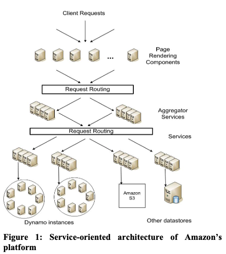
A simple consistent-hash ring:
```python id=”consistent-hash-ring” import bisect from dataclasses import dataclass
@dataclass(frozen=True) class RingPoint: token: int node_id: str
class ConsistentHashRing: def init(self, virtual_nodes_per_node: int = 128): self.virtual_nodes_per_node = virtual_nodes_per_node self.points: list[RingPoint] = [] self.tokens: list[int] = []
def add_node(self, node_id: str) -> None:
    for i in range(self.virtual_nodes_per_node):
        token = stable_hash(f"{node_id}:{i}")
        self.points.append(RingPoint(token=token, node_id=node_id))

    self.points.sort(key=lambda point: point.token)
    self.tokens = [point.token for point in self.points]

def remove_node(self, node_id: str) -> None:
    self.points = [point for point in self.points if point.node_id != node_id]
    self.points.sort(key=lambda point: point.token)
    self.tokens = [point.token for point in self.points]

def owner(self, key: str) -> str:
    if not self.points:
        raise ValueError("ring has no nodes")

    token = stable_hash(key)
    index = bisect.bisect_left(self.tokens, token)

    if index == len(self.points):
        index = 0

    return self.points[index].node_id ```
Dynamo used MD5 to generate a 128-bit key identifier and consistent hashing to determine which storage nodes were responsible for a key. It also assigned each physical node to multiple positions on the ring through virtual nodes to reduce imbalance and support heterogeneity. The Dynamo paper states that virtual nodes let load from an unavailable node disperse across remaining nodes and let a new node accept a roughly equivalent amount of load from available nodes.
A real Cassandra-style example is similar. Cassandra maps nodes to one or more tokens on a continuous hash ring, hashes the partition key to a token, then walks the ring to find the replica set. Its documentation explicitly says this reduces remapping compared with naive modulo hashing and describes an example with replication factor \(3\) where the system walks the ring until it finds three distinct nodes.
```python id=”ring-replica-selection” def replicas_for_key(ring: ConsistentHashRing, key: str, replication_factor: int) -> list[str]: token = stable_hash(key) index = bisect.bisect_left(ring.tokens, token)
replicas = []
seen = set()

while len(replicas) < replication_factor:
    point = ring.points[index % len(ring.points)]

    if point.node_id not in seen:
        replicas.append(point.node_id)
        seen.add(point.node_id)

    index += 1

return replicas ```
The important implementation detail is that “walk the ring” should choose distinct failure domains when the replication policy requires it. In a multi-zone cluster, choosing three adjacent virtual nodes is not enough if all three map to the same rack or availability zone.
Virtual nodes
Virtual nodes, or vnodes, split a physical node’s ownership into many small ranges. Instead of node \(A\) owning one large interval on the ring, it owns many small intervals spread around the ring. This improves load balance and makes incremental scaling easier because each physical node can receive or give away many small pieces.
DataStax’s Cassandra documentation describes the transition from one token per node to vnodes: in Cassandra 1.2 and later, each node can have many tokens, and vnodes let a node own many small partition ranges distributed throughout the cluster. It also notes the operational tradeoff that more tokens can increase peer sharing and must be balanced against reads and writes.
A placement table with vnodes:
```python id=”vnode-placement” @dataclass(frozen=True) class TokenRange: start: int end: int node_id: str
def ranges_owned_by_node(ranges: list[TokenRange], node_id: str) -> list[TokenRange]: return [r for r in ranges if r.node_id == node_id]
def move_range(range_id: int, source: str, destination: str): stream_data(range_id, source=source, destination=destination) update_ring_metadata(range_id, new_owner=destination)
Vnodes reduce the variance in ownership size. If each physical node owns $$m$$ independently placed virtual ranges, the relative imbalance tends to decrease as $$m$$ increases, though real systems must account for non-uniform key popularity, replica placement, streaming overhead, repair cost, and failure-domain constraints.
A useful rule of thumb is:
$$
\text{more vnodes} \Rightarrow \text{better balance but more metadata and more repair or streaming fanout}.
$$
### Range partitioning
Range partitioning stores ordered keys in contiguous intervals. A range might contain all keys from `user:1000` through `user:1999`, or all SQL rows whose primary keys fall between two boundary keys. Range partitioning is natural for ordered scans, prefix queries, time-series windows, and SQL indexes. The cost is that sequential or skewed keys can create hotspots.
Bigtable is the canonical range-partitioned storage example. A Bigtable is a sorted map indexed by row key, column key, and timestamp; each table is split into tablets, and each tablet contains the data for a row range. The paper states that a table starts as one tablet and is automatically split into multiple tablets as it grows, with tablets around 100 to 200 MB by default.
The following figure ([source](https://research.google.com/archive/bigtable-osdi06.pdf)) shows Figure 4, “Tablet location hierarchy,” where a Chubby file points to the root tablet, the root tablet points to METADATA tablets, and METADATA tablets point to user tablets.
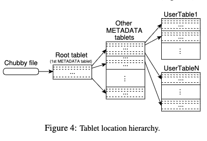
A simplified range router:
```python id="range-router"
@dataclass(frozen=True)
class RangeDescriptor:
start_key: str
end_key: str
range_id: str
leaseholder: str
class RangeMap:
def __init__(self, ranges: list[RangeDescriptor]):
self.ranges = sorted(ranges, key=lambda r: r.start_key)
def lookup(self, key: str) -> RangeDescriptor:
for descriptor in self.ranges:
if descriptor.start_key <= key < descriptor.end_key:
return descriptor
raise KeyError(f"no range for key {key}")
CockroachDB uses a similar range abstraction for SQL data. Its documentation says the keyspace is divided into contiguous chunks called ranges, every key is found in one range, ranges split as they reach the default size, each range has replicas, and a range leaseholder coordinates read and write requests for that range.
```python id=”range-read-write-routing” def route_sql_write(key, statement): descriptor = range_cache.lookup(key)
try:
    return send_to_node(descriptor.leaseholder, statement)
except NotLeaseholder as error:
    range_cache.update(error.current_descriptor)
    return send_to_node(error.current_descriptor.leaseholder, statement) ```
Range partitioning gives efficient scans:
```python id=”range-scan” def scan(start_key: str, end_key: str): current = start_key results = []
while current < end_key:
    descriptor = range_cache.lookup(current)
    batch = send_to_node(
        descriptor.leaseholder,
        {
            "type": "Scan",
            "start_key": current,
            "end_key": min(end_key, descriptor.end_key),
        },
    )

    results.extend(batch.rows)
    current = descriptor.end_key

return results ```
The tradeoff is that range scans may touch many range owners, and sequential inserts can hammer the last range.
Hash partitioning versus range partitioning
Hash partitioning spreads keys evenly when the hash input has high cardinality. Range partitioning preserves ordering and enables efficient scans. The choice should follow access patterns.
| Requirement | Better fit | Reason |
|---|---|---|
| Point lookups by user ID | Hash partitioning | Spreads load evenly |
| Ordered scan by timestamp | Range partitioning | Reads adjacent records efficiently |
| Per-customer transactions | Hash by customer ID | Keeps customer state together |
| SQL primary-key range scans | Range partitioning | Supports ordered indexes |
| Time-series ingestion | Hash or bucketed range | Avoids newest-time hotspot |
| Event stream per aggregate | Hash by aggregate ID | Preserves per-aggregate order |
| Search index shards | Hash or term/routing based | Balances query and indexing load |
| Object store prefixes | Prefix-aware distribution | Scales requests across prefixes |
A concrete AWS example is DynamoDB. The partition key is central to workload distribution, and AWS recommends designing for uniform activity across partition keys. The same documentation states that every DynamoDB partition is designed to deliver up to 3,000 read capacity units or 1,000 write capacity units per second, with item size affecting how many actual operations those units support.
Bad DynamoDB key design:
```python id=”bad-dynamodb-key-design”
All writes for the day hit one logical partition key.
partition_key = f”orders#{today_date()}” sort_key = order_id
Better write-sharded design:

```python id="dynamodb-write-sharding"
def partition_key_for_order(order_id: str, date: str, shard_count: int = 200) -> str:
    shard = stable_hash(order_id) % shard_count
    return f"orders#{date}#{shard:03d}"

item = {
    "PK": partition_key_for_order(order_id, "2026-07-04"),
    "SK": order_id,
    "amount_cents": 4200,
}
AWS’s Using write sharding to distribute workloads evenly in your DynamoDB table describes the same idea: add a random or calculated suffix to expand the partition-key space, improving write parallelism, while reads may need to query all suffixes and merge results unless the suffix is calculable from a lookup attribute.
Hot partitions
A hot partition is a partition whose request rate, storage growth, CPU cost, lock contention, or fanout is much higher than the rest. Partitioning by itself does not solve skew. A single celebrity user, tenant, product, stock ticker, viral post, popular object, or current timestamp can overload one partition.
A simple skew metric is:
\[\text{skew} = \frac{\max_i Q_i}{\frac{1}{N}\sum_{i=1}^{N} Q_i}.\]If skew is near \(1\), load is balanced. If skew is \(50\), one partition is doing fifty times average load.
```python id=”hot-partition-detector” def detect_hot_partitions(qps_by_partition: dict[str, float], threshold: float = 5.0): average = sum(qps_by_partition.values()) / len(qps_by_partition)
return [
    partition
    for partition, qps in qps_by_partition.items()
    if qps / max(average, 1.0) >= threshold
] ```
DynamoDB has service-side mitigations for some hot-partition patterns. AWS’s DynamoDB burst and adaptive capacity says adaptive capacity automatically increases throughput for partitions receiving more traffic when table-level capacity and per-partition limits allow it. It also says adaptive capacity can isolate frequently accessed items so they do not reside on the same partition, but a consistently hot single item can still be limited by the partition maximum.
The following figure (source) shows DynamoDB adaptive capacity increasing throughput for a hot partition so partition 4 can sustain higher write traffic without throttling.
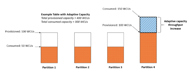
Application-level mitigations are still required when the logical key itself is hot:
| Hotspot source | Example | Mitigation |
|---|---|---|
| Current timestamp | events#2026-07-04T19:00 |
Add hash bucket, then merge on read |
| Single tenant | One huge enterprise customer | Tenant subshards or dedicated tenant placement |
| Celebrity user | One profile receives huge reads | Cache, fanout, read replicas, object CDN |
| Popular counter | One post like-count | Sharded counters and async aggregation |
| Monotonic ID | Auto-increment primary key | Hash prefix, UUID, sequence block allocation |
| Single queue partition | One event key dominates | Split key or relax per-key ordering |
| Large item collection | One partition key has huge sort-key set | Bucket sort key or split collection |
A sharded counter:
```python id=”sharded-counter” def increment_counter(counter_id: str, shard_count: int = 64): shard = random_int(0, shard_count - 1)
db.update(
    key=f"counter#{counter_id}#{shard}",
    operation="ADD count 1",
)
def read_counter(counter_id: str, shard_count: int = 64) -> int: total = 0
for shard in range(shard_count):
    total += db.get(f"counter#{counter_id}#{shard}").count

return total ```
This improves write throughput at the cost of read fanout and possibly stale aggregation. It is a good fit for likes, views, metrics, and approximate counters, but not for account balances unless paired with stronger invariant management.
Time-series partitioning
Time-series data is especially prone to hotspots because new writes often target the newest time bucket. A naive partition key like date or hour sends all current writes to one partition.
Bad design:
```python id=”bad-time-series-key” partition_key = f”metrics#{current_hour()}” sort_key = f”{timestamp_ms()}#{host_id}”
Better design with time bucket plus hash bucket:

```python id="bucketed-time-series-key"
def metric_key(metric_name: str, host_id: str, timestamp_ms: int):
    hour = timestamp_ms // (60 * 60 * 1000)
    bucket = stable_hash(host_id) % 128

    return {
        "PK": f"metric#{metric_name}#hour#{hour}#bucket#{bucket}",
        "SK": f"{timestamp_ms}#{host_id}",
    }
A query for one hour now fans out over 128 buckets:
```python id=”bucketed-time-series-query” def query_metric_hour(metric_name: str, hour: int): results = []
for bucket in range(128):
    results.extend(
        db.query(
            pk=f"metric#{metric_name}#hour#{hour}#bucket#{bucket}"
        )
    )

return merge_sorted(results, key=lambda row: row["timestamp_ms"]) ```
This is the same tradeoff AWS highlights in DynamoDB write sharding: random or calculated suffixes distribute writes, but broad reads must query multiple suffixes and merge the results unless the suffix can be derived from the query.
Object stores have a related prefix-based version of this issue. Amazon S3 documentation says applications can achieve at least 3,500 write-style requests and 5,500 read-style requests per second per partitioned prefix, and can increase throughput by parallelizing across prefixes. It also says scaling happens gradually and workloads may see temporary 503 Slow Down responses while S3 adapts.
A high-throughput S3 layout might spread objects across prefixes:
```python id=”s3-prefix-sharding” def s3_key(tenant_id: str, object_id: str, timestamp_ms: int): prefix_bucket = stable_hash(object_id) % 256 day = timestamp_ms // (24 * 60 * 60 * 1000)
return f"tenant={tenant_id}/day={day}/bucket={prefix_bucket:03d}/{object_id}.json" ```
The key point is that partitioning affects both storage and request routing. A layout that is convenient for humans may be bad for throughput, and a layout that is great for writes may make reads more expensive.
Tenant partitioning
Multi-tenant systems often consider partitioning by tenant. This is attractive because tenant data is naturally isolated, billing and quotas are tenant-scoped, and per-tenant backup or deletion is easier. The risk is tenant skew: one large tenant may dwarf all others.
Three common patterns:
| Pattern | How it works | Good for | Risk |
|---|---|---|---|
| Shared partitions | Many tenants mixed by hash | Small tenants, high utilization | Harder isolation |
| Tenant-as-partition | One tenant maps to one shard or range | Medium tenants, tenant-local queries | Large tenant hotspot |
| Dedicated tenant placement | Large tenants get their own shards or clusters | Enterprise isolation | Operational overhead |
A hybrid router:
```python id=”tenant-aware-routing” def route_tenant_request(tenant_id: str, key: str): placement = tenant_catalog.get(tenant_id)
if placement.mode == "dedicated":
    return placement.cluster

if placement.mode == "subsharded":
    subshard = stable_hash(key) % placement.subshard_count
    return placement.subshards[subshard]

shared_shard = stable_hash(tenant_id) % SHARED_SHARD_COUNT
return shared_clusters[shared_shard] ```
CockroachDB’s data placement model is a real SQL example of locality-aware placement. Its documentation defines ranges, replicas, and leaseholders, and its replication controls say CockroachDB can use locality to move range leases closer to current workload, reducing network round trips and improving read performance.
Shard keys and access patterns
A shard key is the field or set of fields used to decide placement. The best shard key has high cardinality, uniform access, stable value, and alignment with the most important queries and transactions.
A poor shard key creates fanout:
```sql id=”scatter-query” select * from orders where status = ‘PENDING’ order by created_at limit 100;
If `orders` is sharded by `customer_id`, this query must ask every shard for its pending orders, then merge the top results. This is called scatter-gather. It may be acceptable for administrative tools, but it is dangerous on hot user-facing paths.

A shard-key-aligned query:

```sql id="single-shard-query"
select *
from orders
where customer_id = 'cus_123'
order by created_at desc
limit 100;
If customer_id is the shard key, this routes to one shard. The implementation difference is large:
```python id=”single-shard-vs-scatter” def get_orders_for_customer(customer_id): shard = shard_for_customer(customer_id) return shard.query(“select * from orders where customer_id = ?”, [customer_id])
def get_pending_orders_global(): partials = []
for shard in all_shards():
    partials.append(
        shard.query(
            "select * from orders where status = 'PENDING' order by created_at limit 100"
        )
    )

return merge_top_k(partials, k=100, key=lambda row: row.created_at) ```
| Vitess is a concrete MySQL ecosystem example. Vitess supports horizontal sharding, uses vindexes to map rows to keyspace IDs and shards, and supports live resharding by copying data from source shards to destination shards, catching up on replication, comparing for integrity, shifting serving traffic, and deleting source shards. [The Vitess Docs | Shard](https://vitess.io/docs/archive/22.0/concepts/shard/) describes this resharding flow, and PlanetScale’s Sharding with PlanetScale explains that VTGate routes queries to the appropriate MySQL instances so applications can see the sharded database as a unified system. |
```python id=”vitess-style-routing” def route_query(sql, bind_vars): vindex = lookup_vindex_for_table(sql.table)
if vindex.can_route(bind_vars):
    keyspace_id = vindex.map(bind_vars[vindex.column])
    shard = shard_for_keyspace_id(keyspace_id)
    return vtgate_send(shard, sql, bind_vars)

return scatter_to_all_shards(sql, bind_vars) ```
The product lesson is that sharding is not just storage placement. It changes query planning, schema design, secondary indexes, migrations, backfills, online DDL, and application access patterns.
Secondary indexes in sharded systems
Secondary indexes are difficult because the primary shard key and the secondary lookup key may not align. Suppose user rows are sharded by user_id, but the application needs lookup by email.
Option 1: Global secondary index
```python id=”global-secondary-index” def create_user(user_id, email, profile): user_shard = shard_for_user_id(user_id) index_shard = shard_for_email(email)
with distributed_transaction() as tx:
    tx.put(user_shard, f"user#{user_id}", profile)
    tx.put(index_shard, f"email#{email}", user_id) ```
This supports efficient email lookup but requires cross-shard coordination for correctness.
Option 2: Local secondary index
```python id=”local-secondary-index” def create_user(user_id, email, profile): shard = shard_for_user_id(user_id)
with shard.transaction() as tx:
    tx.put(f"user#{user_id}", profile)
    tx.put(f"local_email_index#{email}", user_id) ```
This is cheap to write but cannot find an arbitrary email without searching every shard.
Option 3: Asynchronous global index
```python id=”async-global-index” def create_user(user_id, email, profile): shard = shard_for_user_id(user_id)
with shard.transaction() as tx:
    tx.put(f"user#{user_id}", profile)
    tx.insert_outbox({
        "type": "UserEmailIndexed",
        "email": email,
        "user_id": user_id,
    })
def index_consumer(event): index_shard = shard_for_email(event[“email”]) index_shard.put(f”email#{event[‘email’]}”, event[“user_id”])
This is scalable but eventually consistent. The API must decide whether email uniqueness is strongly enforced at write time or eventually repaired. A login path usually needs a strongly consistent or carefully fenced unique index. A search path can often tolerate asynchronous indexing.

### Cross-shard transactions

A single-shard transaction is much simpler than a cross-shard transaction. If all rows touched by a transaction live on one shard, the shard’s local database can provide atomicity and isolation. If a transaction touches several shards, the system needs two-phase commit, consensus-backed transaction records, deterministic ordering, saga compensation, escrow, or a weaker contract.

Single-shard transfer:

```python id="single-shard-transaction"
def transfer_between_accounts_same_customer(customer_id, from_account, to_account, amount):
    shard = shard_for_customer(customer_id)

    with shard.transaction() as tx:
        debit(tx, from_account, amount)
        credit(tx, to_account, amount)
Cross-shard transfer:
```python id=”cross-shard-transaction” def transfer_between_customers(from_customer, to_customer, amount): from_shard = shard_for_customer(from_customer) to_shard = shard_for_customer(to_customer)
return two_phase_commit(
    participants=[from_shard, to_shard],
    work=lambda tx: [
        debit(tx.at(from_shard), from_customer, amount),
        credit(tx.at(to_shard), to_customer, amount),
    ],
) ```
The second path has more failure states. The coordinator can crash after one participant prepares. A participant can be locked while waiting for a decision. Network partitions can block completion. This is why many sharded production systems design their shard key around the dominant transactional boundary. For example, if most business operations are per customer, shard by customer. If most operations are per tenant, shard by tenant. If most operations are per order, shard by order.
CockroachDB is a real system that chooses a different approach: it keeps SQL as a distributed abstraction while splitting the keyspace into ranges. Its architecture says each range is replicated, the leaseholder coordinates reads and writes for the range, and Raft logs provide consistent replication. The CockroachDB paper says replicas of a range form a Raft group, and commands are applied after Raft declares them committed.
Rebalancing
Rebalancing moves partitions, shards, ranges, or tablets between nodes to reduce load imbalance, recover from failure, add capacity, or change placement policy. Rebalancing is a distributed-systems problem because the system must move data while reads and writes continue.
A safe migration has phases:
| Phase | Purpose |
|---|---|
| Plan | Choose source, destination, and movement order |
| Copy | Transfer a snapshot of partition data |
| Catch up | Replicate writes that occurred during copy |
| Verify | Compare counts, checksums, or key ranges |
| Cut over | Route new traffic to destination |
| Drain | Stop old owner from serving or forward writes |
| Cleanup | Delete old copy after retention window |
A generic live migration:
```python id=”live-partition-migration” def migrate_partition(partition_id, source, destination): epoch = placement_store.begin_migration(partition_id, source, destination)
snapshot_token = source.start_snapshot(partition_id)
stream_snapshot(source, destination, partition_id, snapshot_token)

while source.change_lag(partition_id, destination) > MAX_CATCHUP_LAG:
    stream_changes(source, destination, partition_id)

if not verify_partition(source, destination, partition_id):
    placement_store.abort_migration(partition_id, epoch)
    raise DataMismatch()

placement_store.cutover(partition_id, destination, epoch)

source.stop_serving(partition_id, epoch)
destination.start_serving(partition_id, epoch)

placement_store.complete_migration(partition_id, epoch) ```
The epoch is essential. If the old owner continues serving writes after cutover, the partition can split brain. Every request should carry the placement epoch or be rejected by stale owners.
```python id=”partition-epoch-check” def handle_partition_request(request): current = placement_store.get(request.partition_id)
if request.epoch != current.epoch:
    raise StalePlacement({
        "current_epoch": current.epoch,
        "request_epoch": request.epoch,
    })

return apply_request(request) ```
Vitess’s documented resharding flow is a concrete example of live migration at the database layer: destination shards receive copied data, catch up on replication, are compared against the source for integrity, then live serving is shifted to destination shards. Bigtable tablet movement is another example: tablet servers can stop serving a tablet and another server can load it using metadata and persistent files.
Splitting and merging partitions
Splitting divides an overloaded or oversized partition. Merging combines small adjacent partitions to reduce metadata and operational overhead. Range-partitioned systems can split at a key boundary. Hash-partitioned systems often split by adding more buckets or by introducing subshards for hot keys.
Range split:
```python id=”range-split” def split_range(range_id, split_key): old = metadata.get_range(range_id)
left = RangeDescriptor(
    start_key=old.start_key,
    end_key=split_key,
    range_id=new_id(),
    leaseholder=old.leaseholder,
)

right = RangeDescriptor(
    start_key=split_key,
    end_key=old.end_key,
    range_id=new_id(),
    leaseholder=choose_leaseholder(),
)

write_split_metadata_atomically(old, left, right) ```
Bigtable’s tablet servers split tablets that grow too large, and the split is committed by recording the new tablet information in the METADATA table; the master can detect missed split notifications later. CockroachDB ranges also split as data grows, with each range replicated and independently placed.
Hash subshard split:
```python id=”hot-key-subshard-split” def subpartition_for_hot_key(logical_key: str, entity_id: str, subshard_count: int): subshard = stable_hash(entity_id) % subshard_count return f”{logical_key}#subshard={subshard}”
This is common for hot tenants, hot counters, large item collections, or high-ingest time buckets. The tradeoff is read fanout and more complicated aggregation.

### Partition routing and metadata

Every partitioned system needs a routing path. The client, proxy, gateway, broker, or coordinator must map a request to the right partition owner.

Routing can live in different places:

| Routing location | Example                         | Benefit                       | Risk                           |
| ---------------- | ------------------------------- | ----------------------------- | ------------------------------ |
| Client library   | Bigtable client tablet cache    | Low latency                   | Stale metadata in many clients |
| Proxy or gateway | Vitess VTGate                   | Centralized logic             | Proxy becomes critical path    |
| Coordinator node | SQL gateway, query planner      | Simpler clients               | Coordinator bottleneck         |
| Broker metadata  | Kafka producer metadata         | Efficient partition targeting | Metadata refresh complexity    |
| Load balancer    | Stateless service shard routing | Simple clients                | Harder per-key control         |

A metadata cache should handle stale routing by retrying with refreshed metadata:

```python id="routing-cache-refresh"
def send_partition_request(key, request):
    descriptor = routing_cache.lookup(key)

    try:
        return send(descriptor.owner, request)
    except WrongOwner as error:
        routing_cache.update(error.correct_descriptor)
        return send(error.correct_descriptor.owner, request)
Bigtable clients cache tablet locations, and if a cached location is wrong, they move up the tablet-location hierarchy to rediscover the correct tablet server. The paper states that an empty client cache requires three network round trips, including one Chubby read, and that stale entries can require more.
Partition ownership, leases, and fencing
A partition owner is the node allowed to serve reads, writes, or both for that partition. Ownership needs a term, epoch, lease, or generation to avoid stale owners.
```python id=”partition-owner-record” @dataclass(frozen=True) class PartitionOwner: partition_id: str owner_node: str epoch: int lease_expires_at_ms: int | None
A safe owner check:

```python id="owner-fencing-check"
def write_partition(request):
    owner = placement_store.get_owner(request.partition_id)

    if request.owner_epoch != owner.epoch:
        raise StaleOwner()

    if request.sender != owner.owner_node:
        raise NotOwner()

    storage.write(request.key, request.value, fencing_epoch=request.owner_epoch)
CockroachDB uses range leaseholders. Its documentation states that the leaseholder coordinates all read and write requests for a range, and that for most tables and queries the leaseholder is the only replica that can serve consistent reads. The CockroachDB paper explains that lease acquisition is committed through Raft to prevent overlapping leases, which is exactly the fencing problem in range form.
Placement and failure domains
Partition placement decides which nodes store each partition or replica. A placement policy should consider capacity, load, failure domains, compliance, latency, hardware type, and maintenance state.
A simple placement policy:
```python id=”placement-policy” def choose_replicas(nodes, replication_factor, required_zones): candidates = [ node for node in nodes if node.healthy and node.free_disk_gb > MIN_FREE_DISK_GB ]
chosen = []
used_zones = set()

for zone in required_zones:
    node = least_loaded([n for n in candidates if n.zone == zone])
    chosen.append(node)
    used_zones.add(zone)

while len(chosen) < replication_factor:
    node = least_loaded([
        n for n in candidates
        if n not in chosen and n.zone not in used_zones
    ])
    chosen.append(node)
    used_zones.add(node.zone)

return chosen ```
Real systems encode this in different ways. CockroachDB supports manual and automatic replica placement, including locality and constraints for regions and availability zones. Cassandra replication strategies can place replicas across racks and datacenters. Dynamo’s original system used preference lists and virtual nodes so each key mapped to a set of storage nodes.
A useful placement invariant is:
\[\forall p,\ \text{replicas}(p) \text{ must not all share the same failure domain}.\]Examples:
| Partition type | Placement requirement |
|---|---|
| Critical metadata shard | Spread across three zones, quorum available under one-zone loss |
| Hot tenant shard | Place near tenant’s primary region and isolate from noisy neighbors |
| Kafka topic partition | Assign leader and replicas across brokers and racks |
| Search index shard | Spread primary and replica shards across nodes |
| Object-store prefix | Spread request load across partitioned prefixes |
| GPU inference shard | Place model replicas near GPU memory and routing layer |
Partitioning in event streams
Kafka partitions are a clean example of partitioning work and data together. A topic is split into partitions. Each partition is an ordered log. Producers choose a partition, often by key. Consumers in a group divide partitions among themselves. This means maximum consumer parallelism for a topic is bounded by partition count.
If a topic has \(P\) partitions and one consumer group has \(C\) consumers, then useful parallelism is roughly:
\[\min(P, C).\]```python id=”kafka-partition-assignment” def assign_partitions(partitions: list[int], consumers: list[str]) -> dict[str, list[int]]: assignment = {consumer: [] for consumer in consumers}
for index, partition in enumerate(partitions):
    consumer = consumers[index % len(consumers)]
    assignment[consumer].append(partition)

return assignment ```
The design tradeoff is that per-key order and parallelism compete. If all events use the same key, they all go to one partition and one consumer processes them in order. If events use many keys, load spreads, but operations across keys are not globally ordered. Kafka’s documentation and Confluent’s partition-key guide both emphasize that same-key events go to the same partition, which is the mechanism behind per-key ordering.
A common event-stream design:
```python id=”event-key-choice”
Preserves order for one order.
producer.send( topic=”order-events”, key=order_id, value={“type”: “OrderPaid”, “order_id”: order_id}, )
Preserves order for one customer, but may hotspot large customers.
producer.send( topic=”customer-events”, key=customer_id, value={“type”: “CustomerProfileUpdated”, “customer_id”: customer_id}, )
The correct key depends on the invariant. If order lifecycle events must be processed in order, key by `order_id`. If all customer events must be ordered, key by `customer_id`. If one customer can become hot, split by customer plus subkey and accept weaker ordering where safe.

### Partitioning in distributed SQL systems

Distributed SQL systems often combine range partitioning, replication, MVCC, and distributed transactions. CockroachDB is a concrete example. User data and indexes are stored in a sorted key-value map divided into ranges. Each range has replicas, each range uses Raft for consensus, and a leaseholder coordinates consistent reads and writes for that range.

A simplified SQL-to-range execution path:

```python id="distributed-sql-range-planning"
def execute_select_by_primary_key(table, primary_key):
    key = encode_sql_primary_key(table, primary_key)
    descriptor = range_cache.lookup(key)

    return send_to_node(
        descriptor.leaseholder,
        {
            "type": "KVGet",
            "key": key,
            "timestamp": transaction_timestamp(),
        },
    )
A range scan may involve many ranges:
```python id=”distributed-sql-range-scan” def execute_range_query(table, start_pk, end_pk): start_key = encode_sql_primary_key(table, start_pk) end_key = encode_sql_primary_key(table, end_pk)
spans = range_cache.spans_for(start_key, end_key)

partials = [
    send_to_node(span.leaseholder, {"type": "KVScan", "span": span})
    for span in spans
]

return merge_ordered(partials) ```
This gives SQL users a unified database abstraction, but the underlying distributed plan still depends on partition count, leaseholder placement, cross-range transaction cost, range splits, and network latency.
Partitioning in application-sharded databases
Many companies start with application-level sharding before adopting a system like Vitess or distributed SQL. The application owns a shard map and routes queries directly.
```python id=”application-shard-map” SHARDS = { 0: “mysql-000.example.com”, 1: “mysql-001.example.com”, 2: “mysql-002.example.com”, 3: “mysql-003.example.com”, }
def shard_for_user(user_id: str) -> int: return stable_hash(user_id) % len(SHARDS)
def get_connection_for_user(user_id: str): shard_id = shard_for_user(user_id) return mysql_connect(SHARDS[shard_id])
This is simple at first, but it leaks sharding into application code. Every query must know the shard key. Cross-shard joins become application logic. Resharding is custom. Global secondary indexes become custom. Backfills need shard-aware orchestration. PlanetScale’s Vitess material describes the operational motivation for moving this logic into Vitess and VTGate: VTGate acts as the entry point and routes queries to the appropriate MySQL instances, keeping sharding complexity out of application logic.

### Global IDs and shard-aware identifiers

Partitioned systems need identifiers that do not create hotspots and can be generated safely across nodes. Auto-incrementing IDs are simple but can concentrate writes on the newest range and require central coordination.

Common ID strategies:

| Strategy                   | Benefit                                | Risk                                         |
| -------------------------- | -------------------------------------- | -------------------------------------------- |
| Auto-increment             | Human-friendly, compact                | Central bottleneck and range hotspot         |
| UUIDv4                     | Distributed generation and good spread | Poor locality                                |
| Time-sortable UUID or ULID | Rough time order                       | Can hotspot if used directly as range key    |
| Snowflake-style ID         | Time plus worker plus sequence         | Requires worker ID assignment and clock care |
| Shard-prefixed ID          | Easy routing                           | Leaks topology and complicates resharding    |

A Snowflake-style sketch:

$$
ID = (timestamp \ll a) \mid (worker_id \ll b) \mid sequence.
$$

```python id="snowflake-style-id"
def generate_id(timestamp_ms: int, worker_id: int, sequence: int) -> int:
    return (
        (timestamp_ms << 22)
        | (worker_id << 12)
        | sequence
    )
If the ID is used as a range-partitioned primary key, time ordering can still make the newest range hot. A common mitigation is to separate identity from placement: use a stable ID for object identity, but use a hash or tenant key for physical placement.
```python id=”identity-vs-placement” order_id = generate_order_id() placement_key = stable_hash(customer_id) % logical_partition_count primary_key = f”partition={placement_key}#order={order_id}”
### Directory-based partitioning

Directory-based partitioning uses a metadata service to map keys, tenants, ranges, or shards to owners. It is more flexible than pure hashing because the control plane can move arbitrary partitions. The cost is a metadata dependency.

```python id="directory-based-partitioning"
class PlacementDirectory:
    def lookup(self, key: str) -> RangeDescriptor:
        return self.find_range_containing(key)

    def move(self, range_id: str, new_owner: str, expected_epoch: int):
        with self.transaction() as tx:
            current = tx.get(range_id)

            if current.epoch != expected_epoch:
                raise ConcurrentPlacementChange()

            tx.put(range_id, current.with_owner(new_owner, epoch=current.epoch + 1))
Bigtable’s tablet hierarchy is a directory-based design: Chubby stores the root tablet location, the root tablet stores locations for METADATA tablets, and METADATA tablets store user tablet locations. Clients cache locations but recover by walking the hierarchy. CockroachDB also has range descriptors and range caches for routing SQL/KV requests.
Directory-based partitioning is common when partitions split and move dynamically. Pure hashing is common when key distribution and node membership are stable enough that deterministic routing is sufficient.
Resharding without downtime
Resharding changes the number or boundaries of shards while the system remains live. It is one of the hardest operational parts of sharding because it combines data copy, live writes, routing changes, consistency checks, and rollback.
A robust resharding process:
```python id=”resharding-state-machine” class ReshardingState: PLANNED = “planned” COPYING = “copying” CATCHING_UP = “catching_up” VERIFYING = “verifying” DUAL_SERVING = “dual_serving” CUTTING_OVER = “cutting_over” COMPLETE = “complete” ABORTED = “aborted”
A staged flow:

```python id="resharding-flow"
def reshard(source_shards, destination_shards):
    job = create_resharding_job(source_shards, destination_shards)

    job.transition("copying")
    copy_snapshot(source_shards, destination_shards)

    job.transition("catching_up")
    replicate_incremental_changes(source_shards, destination_shards)

    job.transition("verifying")
    verify_checksums(source_shards, destination_shards)

    job.transition("cutting_over")
    freeze_or_forward_writes(source_shards)
    update_routing(destination_shards)
    unfreeze_writes(destination_shards)

    job.transition("complete")
    schedule_source_cleanup(source_shards)
Vitess’s documented live resharding process follows this shape: copy data into destination shards, let destination shards catch up on replication, compare against the original to ensure integrity, then shift serving to destination shards and delete source shards.
The hardest edge cases are writes during cutover, long-running transactions, stale clients, partially copied rows, backfill retries, foreign-key-like relationships across shards, and queries that scatter across both old and new layouts. A practical resharding system therefore needs idempotent copy, resumable jobs, checksums, epochs, dual-read or compare modes, and a rollback strategy.
Partition-aware observability
Partitioned systems need per-partition visibility. Cluster-level averages hide the exact problems partitioning creates.
Important metrics:
| Metric | Why it matters |
|---|---|
| QPS per partition | Detect hot partitions |
| p95 and p99 latency per partition | Detect localized overload |
| bytes stored per partition | Detect storage imbalance |
| write rate per partition | Detect ingest hotspots |
| replication lag per partition | Detect unsafe failover candidates |
| owner changes per partition | Detect churn |
| split and merge rate | Detect unstable boundaries |
| migration backlog | Detect rebalancing debt |
| scatter-gather fanout | Detect expensive queries |
| throttles per partition key | Detect bad key design |
A partitioned metric emitter:
```python id=”partitioned-metrics” def record_request(partition_id, operation, latency_ms, status): metrics.increment( “partition.request.count”, tags={ “partition”: partition_id, “operation”: operation, “status”: status, }, )
metrics.histogram(
    "partition.request.latency_ms",
    latency_ms,
    tags={
        "partition": partition_id,
        "operation": operation,
    },
) ```
DynamoDB users see this problem as throttling or hot keys. Kafka users see it as one partition lagging while others are idle. CockroachDB users see it as a hot range or leaseholder. Cassandra users see it as token-range imbalance or hot partitions. S3 users see it as prefix-level scaling behavior and temporary 503 Slow Down responses during scaling.
Query planning over partitions
Partitioning changes query cost. A query that targets one partition can be cheap. A query that targets all partitions can be expensive and fragile.
Cost model:
\[L_{\text{scatter}} \approx \max_i L_i + L_{\text{merge}} + L_{\text{coordination}}.\]If a query hits \(N\) partitions and each partition has independent probability \(p\) of completing under a latency target, the probability that all finish under that target is:
\[P(\text{all fast}) = p^N.\]This is why broad fanout worsens tail latency. A query planner should minimize partition fanout and push filters down to partition owners.
```python id=”partition-aware-query-plan” def plan_query(query): if query.has_equality_filter_on_shard_key(): shard = shard_for_value(query.shard_key_value) return SingleShardPlan(shard=shard, query=query)
if query.has_range_filter_on_primary_key():
    ranges = range_cache.spans_for(query.start_key, query.end_key)
    return RangeScanPlan(ranges=ranges, query=query)

return ScatterGatherPlan(shards=all_shards(), query=query) ```
A production system should treat scatter-gather as a budgeted resource. It should limit maximum fanout, require pagination, push down top-\(k\) filters, use timeouts, and degrade gracefully.
Partitioning and caches
Distributed caches commonly use consistent hashing so clients can route keys to cache nodes directly. The same idea appears in Memcached client libraries, CDN request routing, and application-level read-through caches.
```python id=”cache-consistent-hashing” cache_ring = ConsistentHashRing(virtual_nodes_per_node=256)
for node in cache_nodes: cache_ring.add_node(node.id)
def cache_get(key): node_id = cache_ring.owner(key) return cache_client(node_id).get(key)
When a cache node is added or removed, consistent hashing remaps only a fraction of keys, reducing cache churn. Karger et al.’s consistent hashing work was originally motivated by distributed caching and hot spots on the Web, which is exactly the cache-cluster version of partitioning.

Cache partitioning differs from database partitioning because cache misses are recoverable. A cache can tolerate more movement and weaker consistency than a source-of-truth store. This often justifies simpler routing, lower durability, and faster failover.

### Partitioning and ML/AI serving

Modern AI-serving systems also partition work, though the unit is often model, tenant, request type, GPU, sequence, or KV-cache state rather than database key. A model-serving fleet may shard by model ID, route long-context requests to high-memory GPUs, isolate enterprise tenants, and keep conversational state or KV cache on one worker when reuse matters.

A simplified router:

```python id="ai-serving-routing"
def route_inference_request(request):
    if request.model_size == "large":
        pool = gpu_pools["high_memory"]
    else:
        pool = gpu_pools["standard"]

    if request.kv_cache_session_id:
        sticky = session_directory.lookup(request.kv_cache_session_id)
        if sticky and sticky.healthy:
            return sticky

    return least_loaded(pool.nodes)
This is conceptually the same as data partitioning: choose an ownership unit, route requests to the owner, move ownership when needed, and avoid hotspots. The difference is that the constrained resource may be GPU memory bandwidth, model weights, KV cache, or batch slots rather than disk or rows.
Design checklist for partitioning
- Choose the unit of ownership: Key, range, tablet, shard, partition, tenant, model, queue, or topic partition.
- Match the shard key to invariants: Keep strongly transactional data together when possible.
- Separate logical and physical partitions: Use many movable units rather than one unit per machine.
- Plan for hot keys: Add bucketing, subshards, caching, or dedicated placement before launch.
- Define routing ownership: Decide whether clients, proxies, gateways, or coordinators own routing.
- Version placement metadata: Use epochs so stale owners and stale clients are rejected safely.
- Design for resharding: Copy, catch up, verify, cut over, and clean up should be ordinary workflows.
- Minimize scatter-gather: Make broad fanout explicit, observable, and budgeted.
- Track per-partition metrics: Averages hide skew.
- Place replicas by failure domain: Capacity balance alone is not enough.
- Handle secondary indexes deliberately: Decide whether they are local, global, or asynchronous.
- Avoid monotonic write hotspots: Time, sequence, and auto-increment keys need bucketing or hashing.
- Document staleness: Derived partitions, indexes, and projections need freshness contracts.
- Test migration paths: Rebalancing and resharding should be tested before emergencies.
Common partitioning failure modes
| Failure mode | Cause | Safer design |
|---|---|---|
| One partition throttles while cluster is idle | Hot key or low-cardinality partition key | Write sharding, subshards, cache, dedicated placement |
| Adding a node moves too much data | Naive modulo hashing | Consistent hashing or stable logical partitions |
| Sequential inserts overload last range | Monotonic range key | Hash prefix, bucketed time key, or split policy |
| Query touches every shard | Shard key not aligned with access pattern | Query-specific index, materialized view, or new shard key |
| Rebalancing breaks writes | Old owner still accepts traffic | Placement epochs and fencing |
| Resharding loses data | Copy and live writes not coordinated | Snapshot plus change stream plus verification |
| Secondary lookup is slow | Index key not colocated with primary shard | Global index, local index with scatter, or async projection |
| Cross-shard transaction is slow | Business invariant spans shards | Redesign shard key or use transaction coordinator |
| Range metadata gets stale | Clients cache old owners | Wrong-owner response and metadata refresh |
| Multi-tenant noisy neighbor | Large tenant mixed with small tenants | Tenant isolation, subshards, quotas |
| Too many tiny partitions | Over-splitting | Merge policy and metadata limits |
| Large partition cannot move | Partition unit too coarse | Smaller ranges, tablets, or logical partitions |
Partitioning is the part of distributed systems where abstract scale becomes concrete schema design. The main question is always: “What must be colocated, what can be separated, and what will happen when one key, tenant, range, prefix, or partition becomes much hotter than expected?” Real systems answer this in different ways: Dynamo and Cassandra use token rings and virtual nodes, Bigtable and CockroachDB use sorted ranges that split and move, Kafka uses topic partitions for ordered parallelism, DynamoDB asks users to design high-cardinality partition keys while the service manages physical partitions and adaptive capacity, S3 scales request throughput by prefix, and Vitess hides MySQL shard routing behind VTGate and supports live resharding.
Distributed Storage
Why distributed storage is different from local storage
Distributed storage systems store data across many machines while presenting an interface that looks like files, objects, tables, key-value pairs, blocks, streams, or SQL rows. The core problem is that a local storage engine worries about pages, logs, indexes, checksums, compaction, and crash recovery, while a distributed storage system must additionally handle placement, replication, rebalancing, metadata, stale replicas, node failure, disk failure, network partitions, backup, restore, and operational growth.
A local write path might be:
\[\text{client} \rightarrow \text{WAL} \rightarrow \text{memtable/page cache} \rightarrow \text{disk}.\]A distributed write path might be:
\[\text{client} \rightarrow \text{router} \rightarrow \text{partition owner} \rightarrow \text{replication quorum} \rightarrow \text{local WALs} \rightarrow \text{commit}.\]The key difference is that a distributed storage system must define both local durability and distributed durability. A write acknowledged by one machine may survive a process crash but not a host loss, disk loss, rack loss, or region loss. A write acknowledged by a quorum can survive some replica failures, but may cost more latency. The Google File System by Ghemawat et al. (2003) is a useful early production reference because it separates metadata management in a master from chunk storage in chunkservers, and explicitly designs around component failures as the norm in large clusters.
Storage abstractions
Different distributed storage systems expose different abstractions. The abstraction determines the access pattern, consistency model, metadata design, and failure behavior.
| Abstraction | Interface | Common systems | Typical fit |
|---|---|---|---|
| Distributed filesystem | Files, directories, blocks or chunks | GFS, HDFS, CephFS | Batch processing, large files, shared namespace |
| Object store | Bucket, object key, object bytes, metadata | Amazon S3, Google Cloud Storage, Azure Blob | Data lakes, backups, media, logs, artifacts |
| Key-value store | Key, value, put, get, delete | Dynamo, DynamoDB, Cassandra, RocksDB-backed services | High-scale lookups and writes |
| Wide-column store | Row key, column families, versions | Bigtable, HBase, Cassandra-like models | Sparse structured data, time-series, large tables |
| Distributed SQL | Tables, indexes, transactions, SQL | Spanner, CockroachDB, YugabyteDB | Strong transactions over sharded data |
| Block storage | Volumes, block reads and writes | EBS-style systems, Ceph RBD | VM disks and databases |
| Log storage | Append records, offsets | Kafka, Pulsar, BookKeeper | Streams, event history, replay |
Concrete examples: Amazon S3 exposes object storage with buckets and object keys, and AWS states that S3 now provides strong read-after-write consistency for all applications. HDFS exposes a filesystem where a NameNode manages metadata and DataNodes store blocks. Bigtable exposes a sparse, distributed, persistent multidimensional sorted map indexed by row key, column key, and timestamp.
The storage stack
A distributed storage system is usually layered:
| Layer | Responsibility |
|---|---|
| API layer | Exposes file, object, KV, SQL, or stream interface |
| Routing layer | Maps keys, files, ranges, tablets, objects, or partitions to owners |
| Metadata layer | Stores placement, schema, leases, object metadata, namespace, and versions |
| Replication layer | Copies data or logs across failure domains |
| Local storage engine | Handles WAL, memtable, SSTables, B-trees, pages, compaction, checksums |
| Repair layer | Detects under-replication, divergence, corruption, and missing data |
| Background maintenance | Compaction, garbage collection, rebalancing, snapshots, backups |
| Observability layer | Tracks latency, durability, lag, capacity, errors, and data health |
The local storage engine and distributed replication layer must agree on exactly when a write is durable. For example, a Raft-based range server may not acknowledge a log entry until it is stored durably on a quorum. A local LSM engine may not expose a write as durable until the write-ahead log is flushed. A distributed filesystem may acknowledge a block write only after a replication pipeline has enough copies. These boundaries are where many data-loss bugs occur.
Write-ahead logging
A write-ahead log, or WAL, records intended changes before they are applied to mutable in-memory structures or on-disk data files. The core rule is:
\[\text{log record durable before data page or memtable state is considered durable}.\]If a process crashes after appending to the WAL but before flushing the derived state, recovery replays the WAL. If it crashes before appending the WAL record, the operation is not durable.
```python id=”wal-basic-write” def put(key: bytes, value: bytes): record = encode_record({ “type”: “PUT”, “key”: key, “value”: value, “sequence”: next_sequence_number(), })
wal.append(record)
wal.fsync()

memtable[key] = value
return {"status": "ok"} ```
Recovery:
```python id=”wal-recovery” def recover(): memtable = {}
for record in wal.read_all_valid_records():
    if record.type == "PUT":
        memtable[record.key] = record.value
    elif record.type == "DELETE":
        memtable[record.key] = TOMBSTONE

return memtable ```
A distributed system has at least two log questions: the local storage log and the replication log. In a Raft-backed store, the consensus log is the distributed source of truth, and the local engine may also have its own WAL. Implementations often optimize by integrating these logs, but the correctness requirement remains: acknowledged committed state must survive the failures promised by the durability contract.
fsync, group commit, and durability latency
fsync forces buffered data to stable storage, but it is expensive. Systems therefore batch many writes into one durable flush. This is called group commit.
If one fsync costs \(C_{\text{fsync}}\) and a batch contains \(B\) writes, the fsync cost per write is roughly:
\[C_{\text{per write}} \approx \frac{C_{\text{fsync}}}{B}.\]```python id=”group-commit” class GroupCommitter: def init(self): self.pending = []
def submit(self, record):
    future = Future()
    self.pending.append((record, future))
    return future

def flush_loop(self):
    while True:
        batch = self.take_batch(max_items=1024, max_wait_ms=2)

        if not batch:
            continue

        for record, _future in batch:
            wal.append(record)

        wal.fsync()

        for _record, future in batch:
            future.set_result("durable") ```
The tradeoff is latency. Larger batches improve throughput but make individual writes wait longer. Distributed storage systems add another dimension: the system may batch local WAL writes, replication messages, disk flushes, and client acknowledgements independently. This is why p99 write latency often depends on both network quorum latency and local storage flush behavior.
Checksums and corruption detection
Distributed storage must assume data can be corrupted. Corruption can come from disks, memory, firmware, buggy kernels, torn writes, network transfers, or software bugs. Checksums detect corruption before returning bad data to clients or replicating corrupted data further.
A simple block format:
```python id=”checksummed-block” @dataclass class Block: block_id: str payload: bytes checksum: str
def write_block(block_id: str, payload: bytes): checksum = crc32c(payload) disk.write(block_id, encode(Block(block_id, payload, checksum)))
def read_block(block_id: str) -> bytes: block = decode(disk.read(block_id))
if crc32c(block.payload) != block.checksum:
    raise CorruptBlock(block_id)

return block.payload ```
HDFS has an explicit block-report and replication model. The NameNode receives heartbeats and block reports from DataNodes, and the Apache HDFS architecture guide states that the NameNode makes replication decisions and uses block reports to know which blocks each DataNode stores.
A repair loop:
```python id=”block-repair-loop” def repair_corrupt_block(block_id): healthy_replicas = []
for replica in block_locations(block_id):
    try:
        payload = replica.read(block_id)
        healthy_replicas.append((replica, payload))
    except CorruptBlock:
        mark_replica_bad(block_id, replica)

if not healthy_replicas:
    raise DataLoss(block_id)

source, payload = healthy_replicas[0]

for target in choose_repair_targets(block_id):
    target.write(block_id, payload) ```
Local storage engines: B-trees and LSM trees
Most distributed storage systems depend on local storage engines. Two common families are B-tree-like engines and LSM-tree-like engines.
| Engine family | Write behavior | Read behavior | Good fit |
|---|---|---|---|
| B-tree / B+ tree | Updates pages in place or copy-on-write | Efficient point and range reads | Read-heavy OLTP, stable indexes |
| LSM tree | Writes to WAL and memory, flushes sorted files, compacts later | Reads check memory and multiple sorted files | Write-heavy workloads, high ingest, flash storage |
The LSM-tree design defers random writes by buffering updates in memory and writing sorted runs to disk. The Log-Structured Merge-Tree by O’Neil et al. (1996) introduced the LSM-tree access method for high-update workloads, and RocksDB describes itself as an embeddable persistent key-value store with an LSM design that trades off write amplification, read amplification, and space amplification.
The LSM write path:
```python id=”lsm-write-path” def lsm_put(key, value): seq = next_sequence_number()
wal.append({"seq": seq, "type": "PUT", "key": key, "value": value})
wal.fsync_if_needed()

mutable_memtable.put(key, seq, value)

if mutable_memtable.size_bytes > MEMTABLE_LIMIT:
    freeze_and_schedule_flush(mutable_memtable) ```
The LSM read path:
```python id=”lsm-read-path” def lsm_get(key): value = mutable_memtable.get(key) if value is not NOT_FOUND: return value
for memtable in immutable_memtables:
    value = memtable.get(key)
    if value is not NOT_FOUND:
        return value

for level in levels:
    for sstable in candidate_sstables(level, key):
        if sstable.bloom_filter.might_contain(key):
            value = sstable.get(key)
            if value is not NOT_FOUND:
                return value

return None ```
Concrete examples: Bigtable’s tablet storage design uses a commit log plus memtable and SSTables in GFS. Cassandra uses an LSM-style write path with commit logs, memtables, SSTables, compaction, tombstones, and repair. RocksDB is widely embedded in storage systems that need a local high-performance KV engine. (Bigtable: A Distributed Storage System for Structured Data by Chang et al. (2006) describes the tablet implementation with commit logs, memtables, and SSTables, while Compaction explains that RocksDB compaction algorithms constrain the LSM shape and determine which sorted runs must be read.)
Memtables, SSTables, and Bloom filters
A memtable is an in-memory sorted structure that accepts writes. When it fills, the system freezes it and flushes it to disk as an immutable sorted-string table, often called an SSTable. Because SSTables are immutable, they are simple to write sequentially and safe to reference from snapshots. Reads consult memory first, then disk files.
A simplified flush:
```python id=”memtable-flush” def flush_memtable(memtable): entries = memtable.iter_sorted()
sstable = SSTableWriter(new_file_path())

for key, versions in entries:
    for version in versions:
        sstable.add(key, version.sequence, version.value)

sstable.finish()
install_sstable(sstable.metadata) ```
A Bloom filter is a probabilistic set membership structure. It can say “definitely not present” or “maybe present.” It avoids unnecessary disk reads for keys absent from an SSTable.
False positive probability is commonly approximated by:
\[p \approx \left(1 - e^{-kn/m}\right)^k,\]where \(n\) is number of inserted keys, \(m\) is number of bits, and \(k\) is number of hash functions.
```python id=”bloom-filter-read” def sstable_get(sstable, key): if not sstable.bloom_filter.might_contain(key): return NOT_FOUND
block = sstable.index.find_block(key)
return block.binary_search(key) ```
Bloom filters improve read performance, but they can be tuned incorrectly. Too few bits increase false positives and disk reads. Too many bits waste memory. The RocksDB documentation emphasizes LSM tradeoffs among read amplification, write amplification, and space amplification, which are directly affected by compaction and filter choices.
Compaction
Compaction merges SSTables, removes overwritten values, discards expired versions, and clears tombstones once safe. It is essential because LSM writes create many immutable files.
Without compaction, read amplification grows:
\[\text{read amplification} \approx \text{number of candidate files checked per read}.\]With compaction, background work reduces read amplification but increases write amplification:
\[\text{write amplification} = \frac{\text{bytes written to storage media}}{\text{bytes written by user workload}}.\]A simplified compaction:
```python id=”lsm-compaction” def compact(inputs: list[SSTable]) -> SSTable: iterator = merge_sorted_iterators([table.iter() for table in inputs]) output = SSTableWriter(new_file_path())
for key, versions in group_by_key(iterator):
    live_versions = discard_obsolete_versions(key, versions)

    for version in live_versions:
        output.add(key, version.sequence, version.value)

output.finish()
atomically_replace(inputs, output)
return output ```
RocksDB’s Compaction documentation states that compaction algorithms constrain the LSM tree shape and determine which sorted runs are merged and which sorted runs must be accessed on reads. Universal compaction targets lower write amplification while trading off read and space amplification, according to RocksDB’s Universal Compaction documentation.
Concrete deployment example: Cassandra workloads with many deletes can suffer from tombstone-heavy reads because deleted data must remain until replicas have had time to receive the deletion. LSM systems must coordinate compaction with replication and repair, otherwise one replica may permanently forget a deletion while another still holds the old value.
Tombstones and deletes
Deletes in replicated LSM systems are not immediate physical removals. They are usually written as tombstones, which say “this key or version is deleted.” Tombstones must be retained long enough to propagate to all replicas that may still contain the old value.
```python id=”tombstone-delete” def delete(key): seq = next_sequence_number()
wal.append({"seq": seq, "type": "DELETE", "key": key})
memtable.put(key, seq, TOMBSTONE) ```
A read must treat the newest tombstone as deletion:
```python id=”tombstone-read” def resolve_versions(versions): newest = max(versions, key=lambda version: version.sequence)
if newest.value is TOMBSTONE:
    return None

return newest.value ```
The dangerous bug is resurrection. Suppose replica A receives a delete and compacts away the tombstone too early, while replica B was down and still has the old value. When B returns and anti-entropy repair runs, B can replicate the old value back to A. Production systems therefore use grace periods, repair requirements, version vectors, or consensus to prevent old values from being resurrected.
Distributed filesystems: GFS and HDFS
Distributed filesystems split files into large chunks or blocks and store replicas on many storage nodes. A metadata server tracks namespace, file-to-block mappings, and block locations. Data flows directly between clients and storage nodes where possible.
GFS used a single master for metadata and chunkservers for data. The Google File System by Ghemawat et al. (2003) describes a design optimized for large files, append-heavy workloads, streaming reads, and frequent component failures. HDFS uses a NameNode for filesystem metadata and DataNodes for block storage, and its architecture guide states that the NameNode receives heartbeats and block reports from DataNodes and makes block replication decisions.
The following figure (source) shows the GFS architecture, where clients ask the master for metadata and then read or write file chunks directly with chunkservers.
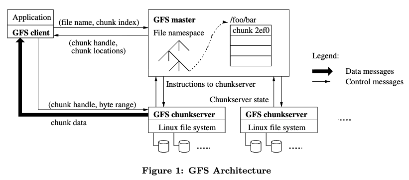
A simplified metadata lookup:
```python id=”distributed-filesystem-lookup” def read_file(path, offset, length): chunks = namenode.lookup_chunks(path, offset, length)
result = b""

for chunk in chunks:
    replica = choose_nearest_healthy_replica(chunk.locations)
    result += replica.read(chunk.chunk_id, chunk.offset, chunk.length)

return result ```
A simplified write pipeline:
```python id=”dfs-write-pipeline” def write_chunk(chunk_id, data, replicas): primary = replicas[0] secondaries = replicas[1:]
# Client streams data to all replicas.
for replica in replicas:
    replica.stage_data(chunk_id, data)

# Primary orders mutation and forwards to secondaries.
primary.commit_mutation(chunk_id, data, secondaries)

wait_for_acks(replicas) ```
GFS’s master is a metadata authority, not the data path for file contents. This design reduces master bandwidth pressure but makes the master’s metadata scalability and availability critical. HDFS has the same broad separation: NameNode metadata and DataNode block storage.
Object storage: S3-style systems
Object stores expose buckets and object keys rather than a POSIX filesystem API. They usually optimize for durability, scale, and simple object operations rather than low-latency small random writes. An object write replaces or creates an object value, and an object read retrieves bytes by key.
Amazon S3 is the most visible example. AWS states that S3 provides strong read-after-write consistency for all applications, including GET, PUT, LIST, and operations that change object tags, ACLs, or metadata. AWS also documents request-rate scaling per prefix, stating that each S3 prefix can support at least 3,500 write-style requests per second and 5,500 read-style requests per second, and that parallelizing across prefixes can increase throughput.
A high-throughput S3 writer should spread load when one prefix is too hot:
```python id=”s3-prefix-distribution” def object_key(tenant_id: str, object_id: str, timestamp_ms: int): day = timestamp_ms // (24 * 60 * 60 * 1000) prefix = stable_hash(object_id) % 256
return f"tenant={tenant_id}/day={day}/prefix={prefix:03d}/{object_id}.json" ```
An object store write path conceptually looks like:
```python id=”object-store-put” def put_object(bucket, key, bytes_value, metadata): object_id = make_object_id(bucket, key) placement = placement_service.choose_replicas(object_id)
version = new_version_id()

for replica in placement.replicas:
    replica.write(object_id, version, bytes_value, metadata)

metadata_store.commit_object_version(
    bucket=bucket,
    key=key,
    version=version,
    replicas=placement.replicas,
    checksum=sha256(bytes_value),
)

return {"version": version} ```
Real cloud object stores are more complex, but this sketch captures the separation between object bytes, object metadata, placement, versioning, and consistency. Object stores are excellent for immutable files, data lakes, logs, checkpoints, images, model artifacts, backups, and batch-processing inputs. They are not a replacement for a low-latency transactional database.
Object placement and CRUSH
Large object stores must decide where replicas or erasure-coded fragments live. A central directory can store every object-to-device mapping, but that metadata can become large and hard to scale. Ceph’s CRUSH algorithm takes a different approach: compute placement deterministically from an object identifier, a cluster map, and placement rules.
CRUSH: Controlled, Scalable, Decentralized Placement of Replicated Data by Weil et al. (2006) presents CRUSH as a pseudo-random deterministic placement function that maps object identifiers to storage devices while respecting a hierarchical cluster map and minimizing unnecessary data movement during cluster changes.
The following figure (source) shows the CRUSH storage hierarchy, where placement rules select devices across failure domains such as rows, cabinets, shelves, and storage devices.
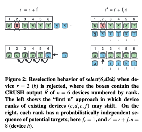
A simplified deterministic placement shape:
```python id=”crush-style-placement” def place_object(object_id, cluster_map, replication_factor): candidates = pseudo_random_walk( seed=stable_hash(object_id), hierarchy=cluster_map.failure_domain_tree, )
replicas = []

for candidate in candidates:
    if satisfies_failure_domain_rules(candidate, replicas):
        replicas.append(candidate)

    if len(replicas) == replication_factor:
        return replicas

raise InsufficientPlacementCandidates() ```
The concrete benefit is that clients and storage nodes can compute placement from shared metadata, rather than asking a central service for every object. The tradeoff is that all participants must have a sufficiently fresh cluster map and placement rules must be carefully designed.
Replication versus erasure coding
Replication stores full copies of data. Erasure coding splits data into fragments and parity fragments so the original can be reconstructed from a subset. Replication is simple and fast for reads and repair, but expensive in storage overhead. Erasure coding is storage-efficient but more complex and often more expensive for small writes and repairs.
For replication factor \(r\):
\[\text{storage overhead} = r.\]For an erasure code with \(k\) data fragments and \(m\) parity fragments:
\[\text{storage overhead} = \frac{k + m}{k}.\]Example:
| Scheme | Can tolerate | Storage overhead |
|---|---|---|
| 3-way replication | 2 replica losses | \(3.0\times\) |
| 6+3 erasure coding | 3 fragment losses | \(1.5\times\) |
| 10+4 erasure coding | 4 fragment losses | \(1.4\times\) |
A simplified erasure-coded write:
```python id=”erasure-coded-write” def write_erasure_coded_object(object_id, data): data_fragments = split_into_k_fragments(data, k=6) parity_fragments = reed_solomon_encode(data_fragments, m=3) fragments = data_fragments + parity_fragments
placements = choose_fragment_placements(object_id, count=9)

for fragment, node in zip(fragments, placements):
    node.write_fragment(object_id, fragment.index, fragment.bytes) ```
Read reconstruction:
```python id=”erasure-coded-read” def read_erasure_coded_object(object_id): fragments = fetch_any_available_fragments(object_id, needed=6)
if len(fragments) < 6:
    raise DataUnavailable(object_id)

return reed_solomon_decode(fragments) ```
Concrete examples: many object and archival storage systems use erasure coding for cold or large objects because storage cost dominates. Hot small objects or metadata are often replicated because read latency and repair simplicity matter more.
Metadata is often the real bottleneck
In storage systems, metadata can be harder than data. Metadata includes namespace, file-to-block mapping, object versions, placement, leases, schemas, range descriptors, tablet locations, permissions, quotas, snapshots, and garbage-collection state.
GFS and HDFS centralize much of the filesystem namespace metadata in a master or NameNode. Bigtable uses a hierarchy where Chubby points to the root tablet, the root tablet points to METADATA tablets, and METADATA tablets point to user tablets. The Bigtable paper explains that this hierarchy lets clients locate tablets and cache tablet locations.
A metadata record for object storage:
```python id=”object-metadata-record” @dataclass class ObjectMetadata: bucket: str key: str version: str size_bytes: int checksum: str replicas: list[str] created_at_ms: int deleted: bool
A metadata lookup:

```python id="metadata-lookup"
def get_object(bucket, key):
    metadata = metadata_store.lookup(bucket, key)

    if metadata is None or metadata.deleted:
        raise NotFound()

    replica = choose_replica(metadata.replicas)
    payload = replica.read(metadata.version)

    if sha256(payload) != metadata.checksum:
        raise CorruptObject(bucket, key)

    return payload
Metadata systems often require stronger consistency than data paths. For example, object bytes can be written to multiple storage nodes, but the namespace update that makes a version visible should be atomic. A stale metadata record can point to missing data. A premature delete can lose data. A bad placement record can make repair copy from the wrong source.
Wide-column storage: Bigtable-style design
Bigtable is a structured distributed storage system built around tablets, SSTables, and a distributed filesystem. Its data model is a sparse multidimensional sorted map:
\[(row,\ column,\ timestamp) \rightarrow value.\]Bigtable: A Distributed Storage System for Structured Data by Chang et al. (2006) is important because it connects storage layout, tablet serving, commit logs, memtables, SSTables, compression, locality groups, and operational scale.
The following figure (source) shows the Bigtable tablet representation, where writes go to a memtable and commit log, and persistent data is stored in immutable SSTables.
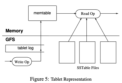
A Bigtable-like write:
```python id=”bigtable-style-write” def put(row_key, column_family, qualifier, timestamp, value): tablet = tablet_locator.lookup(row_key)
mutation = {
    "row": row_key,
    "column": f"{column_family}:{qualifier}",
    "timestamp": timestamp,
    "value": value,
}

return tablet_server(tablet.server).apply_mutation(tablet.id, mutation) ```
A tablet-server local mutation:
```python id=”tablet-server-mutation” def apply_mutation(tablet_id, mutation): commit_log.append({“tablet_id”: tablet_id, “mutation”: mutation}) commit_log.fsync_if_needed()
memtable = tablets[tablet_id].memtable
memtable.put(
    key=(mutation["row"], mutation["column"], mutation["timestamp"]),
    value=mutation["value"],
) ```
Concrete systems: Google Cloud Bigtable is the managed descendant of this family. Apache HBase adopted a Bigtable-like model on top of HDFS. Cassandra is not identical, but shares wide-column and LSM ideas while using Dynamo-style partitioning and replication concepts.
Dynamo-style storage
Dynamo-style systems emphasize availability, partition tolerance, key-value access, consistent hashing, sloppy quorums, hinted handoff, vector clocks, anti-entropy, and application-level conflict resolution. Dynamo: Amazon’s Highly Available Key-value Store by DeCandia et al. (2007) is the production reference, and Cassandra’s architecture documentation explicitly traces parts of its design to Dynamo-style consistent hashing and replication. (Dynamo is relevant here because it shows how a storage system can choose high availability and expose conflict reconciliation rather than forcing every write through a single leader.)
A Dynamo-style write:
```python id=”dynamo-style-write” def put(key, value, context): replicas = replicas_for_key(key, replication_factor=N) version = increment_vector_clock(context.vector_clock, local_node_id)
successes = []

for replica in replicas:
    try:
        replica.store(key, value, version)
        successes.append(replica)
    except Unavailable:
        pass

if len(successes) < W:
    raise Unavailable("write quorum not reached")

return {"vector_clock": version} ```
A Dynamo-style read:
```python id=”dynamo-style-read” def get(key): replicas = replicas_for_key(key, replication_factor=N) responses = []
for replica in replicas:
    try:
        responses.append(replica.read(key))
    except Unavailable:
        pass

if len(responses) < R:
    raise Unavailable("read quorum not reached")

versions = reconcile_by_vector_clock(responses)

if len(versions) > 1:
    return {"conflict": True, "siblings": versions}

return {"conflict": False, "value": versions[0].value} ```
This design is appropriate when availability matters and the application can merge conflicts. It is not appropriate when every operation must have one globally serialized truth at write time.
Concrete AWS distinction: DynamoDB is not simply the Dynamo paper exposed as a service. DynamoDB is a managed database with partition keys, provisioned or on-demand capacity modes, global secondary indexes, transactions, streams, and service-managed physical partitioning. AWS still tells users to design partition keys for uniform load, and documents adaptive capacity for hot partitions. Those are modern managed-service versions of the same physical distribution problem.
Distributed SQL storage
Distributed SQL systems hide sharding behind SQL while using partitioned replicated key-value storage underneath. A SQL table and its indexes are encoded into keys. Those keys are split into ranges or tablets. Each range is replicated. Transactions coordinate reads and writes across one or more ranges.
CockroachDB is a concrete example. Its architecture documentation says data is stored in a monolithic sorted key-value map divided into ranges, each range has replicas, and one replica acts as the leaseholder that coordinates reads and writes. Its paper describes each range as a Raft group, with commands applied after Raft commitment.
A simplified SQL row encoding:
```python id=”sql-to-kv-encoding” def encode_primary_row(table_id: int, primary_key: tuple) -> bytes: return b”/table/” + encode_int(table_id) + b”/primary/” + encode_tuple(primary_key)
def encode_secondary_index(table_id: int, index_id: int, index_key: tuple, primary_key: tuple) -> bytes: return ( b”/table/” + encode_int(table_id) + b”/index/” + encode_int(index_id) + b”/key/” + encode_tuple(index_key) + b”/primary/” + encode_tuple(primary_key) )
A distributed transaction may touch multiple ranges:

```python id="distributed-sql-transaction"
def update_order_and_inventory(tx, order_id, sku, quantity):
    order_key = encode_primary_row(orders_table, (order_id,))
    inventory_key = encode_primary_row(inventory_table, (sku,))

    order = tx.get(order_key)
    inventory = tx.get(inventory_key)

    if inventory["available"] < quantity:
        raise OutOfStock()

    tx.put(order_key, {**order, "status": "confirmed"})
    tx.put(inventory_key, {**inventory, "available": inventory["available"] - quantity})
The storage layer must provide MVCC, timestamp management, conflict detection, replicated range logs, range splits, leaseholder movement, and transaction records. The user sees SQL; the storage system sees ordered keys and replicated ranges.
Snapshots
A snapshot is a consistent view of storage at a point in logical time, transaction timestamp, log index, or version. Snapshots support backups, historical reads, replication catch-up, testing, analytics, and point-in-time recovery.
A snapshot boundary can be:
| Boundary | Example |
|---|---|
| Log index | Raft snapshot at committed index \(i\) |
| MVCC timestamp | Database read as of timestamp \(t\) |
| Filesystem checkpoint | Namespace and block references at checkpoint |
| Object version set | Bucket state at version marker |
| Stream offset set | Consumer snapshot at offsets per partition |
A simple MVCC snapshot read:
```python id=”mvcc-snapshot-read” def read_at_timestamp(key, snapshot_ts): versions = storage.versions_for_key(key)
visible = [
    version for version in versions
    if version.commit_ts <= snapshot_ts and not version.deleted
]

if not visible:
    return None

return max(visible, key=lambda version: version.commit_ts).value ```
Snapshot invariant:
\[\forall x,\ read_{snapshot(t)}(x) = \text{latest committed version of } x \text{ at or before } t.\]A snapshot must keep old versions alive until no active reader, backup, or replication process needs them. This creates garbage-collection pressure. Long-running snapshots can prevent compaction, increase storage usage, and slow reads.
Backup and restore
Backup is not complete until restore has been tested. A backup system must define recovery point objective and recovery time objective:
\[RPO = \text{maximum acceptable data loss window}.\] \[RTO = \text{maximum acceptable time to restore service}.\]A backup process:
```python id=”backup-process” def run_backup(snapshot_ts): manifest = { “snapshot_ts”: snapshot_ts, “ranges”: [], }
for range_descriptor in range_directory.all_ranges():
    files = export_range_at_timestamp(range_descriptor, snapshot_ts)
    checksums = write_files_to_object_store(files)

    manifest["ranges"].append({
        "range_id": range_descriptor.range_id,
        "start_key": range_descriptor.start_key,
        "end_key": range_descriptor.end_key,
        "files": checksums,
    })

object_store.put("backups/manifest.json", json_encode(manifest)) ```
A restore process:
```python id=”restore-process” def restore_backup(manifest): verify_manifest(manifest)
for range_backup in manifest["ranges"]:
    files = fetch_and_verify(range_backup["files"])
    import_range_files(range_backup["start_key"], range_backup["end_key"], files)

rebuild_metadata()
verify_database_consistency() ```
Concrete AWS example: S3 is commonly used as backup storage because it is durable object storage with strong read-after-write consistency and high request-rate scalability when prefixes are designed properly. Database systems often stream backups into object storage, then restore by loading SSTables, range files, WAL archives, or logical dumps.
A serious backup design also needs:
| Concern | Requirement |
|---|---|
| Consistency | Backup corresponds to a valid snapshot |
| Completeness | All ranges, indexes, metadata, and schema are included |
| Integrity | Checksums and manifests are verified |
| Isolation | Backup credentials are separated from production write credentials |
| Retention | Retention policy matches compliance and product needs |
| Restore testing | Automated restore drills validate RPO and RTO |
| Encryption | Data is encrypted in transit and at rest |
| Versioning | Backup format supports software upgrades and downgrades |
Garbage collection
Distributed storage accumulates garbage: old MVCC versions, deleted object versions, tombstones, orphaned blocks, unreferenced SSTables, abandoned multipart uploads, old snapshots, stale replicas, and obsolete metadata. Garbage collection must not delete data that a reader, replica, backup, or recovery process still needs.
A safe deletion condition:
\[\text{delete object } o \iff \text{no live metadata, snapshot, replica repair, or backup references } o.\]Reference-counted garbage collection:
```python id=”reference-count-gc” def garbage_collect_object(object_id): refs = metadata_store.count_references(object_id)
if refs > 0:
    return "still referenced"

if object_id in active_backup_manifest():
    return "needed by backup"

delete_physical_object(object_id)
return "deleted" ```
MVCC garbage collection:
```python id=”mvcc-gc” def gc_versions(key, safe_time): versions = storage.versions_for_key(key)
keep = []
for version in versions:
    if version.commit_ts > safe_time:
        keep.append(version)
    elif is_latest_before_safe_time(version, versions):
        keep.append(version)
    else:
        delete_version(version)

return keep ```
The hard part is computing safe_time. It must account for active transactions, backups, replication, changefeeds, and follower reads. If safe_time moves too far forward, data can be lost. If it moves too slowly, storage bloat grows.
Repair, anti-entropy, and scrubbing
Repair detects and fixes missing, stale, under-replicated, or corrupt data. Scrubbing reads stored data in the background to find latent corruption before all replicas are affected.
A repair loop for replicated blocks:
```python id=”replica-repair” def repair_under_replicated_blocks(): for block_id in metadata_store.blocks(): replicas = metadata_store.live_replicas(block_id)
    if len(replicas) >= desired_replication_factor(block_id):
        continue

    source = choose_healthy_replica(block_id, replicas)
    target = choose_new_replica_target(block_id)

    copy_block(source, target, block_id)
    metadata_store.add_replica(block_id, target) ```
Anti-entropy for key-value replicas:
```python id=”merkle-repair” def repair_range(range_id, replica_a, replica_b): tree_a = replica_a.merkle_tree(range_id) tree_b = replica_b.merkle_tree(range_id)
differing_spans = compare_merkle_trees(tree_a, tree_b)

for span in differing_spans:
    rows_a = replica_a.scan(span)
    rows_b = replica_b.scan(span)
    repaired = reconcile(rows_a, rows_b)

    replica_a.apply_repair(repaired)
    replica_b.apply_repair(repaired) ```
Concrete systems: Cassandra-style systems use repair to synchronize replicas that may have missed updates. HDFS uses block reports and replication management through the NameNode. Object stores and distributed filesystems use background scrubbing to detect corruption and under-replication.
Read repair
Read repair fixes replicas opportunistically during reads. If a quorum read observes stale replicas, it returns the latest value and schedules updates to stale replicas.
```python id=”read-repair” def quorum_get_with_read_repair(key): responses = read_from_replicas(key, count=R) latest = choose_latest_version(responses)
for response in responses:
    if response.version < latest.version:
        send_async(
            response.replica,
            "repair_put",
            key=key,
            value=latest.value,
            version=latest.version,
        )

return latest.value ```
Read repair improves convergence for frequently read data. It does not help cold data, so systems still need background repair or anti-entropy. Read repair also adds write traffic to reads, so it can amplify load during hot-key events.
Storage placement and failure domains
Distributed storage placement must account for correlated failures. A replication factor of three is weak if all three replicas share one rack, zone, power domain, kernel bug, storage controller, or operator action.
Placement invariant:
\[\forall object,\ \text{replicas}(object) \text{ must span required failure domains}.\]A placement rule:
```python id=”failure-domain-placement” def choose_replicas(candidates, replication_factor): chosen = [] used_zones = set() used_racks = set()
for node in sorted(candidates, key=lambda n: n.load):
    if node.zone in used_zones:
        continue
    if node.rack in used_racks:
        continue

    chosen.append(node)
    used_zones.add(node.zone)
    used_racks.add(node.rack)

    if len(chosen) == replication_factor:
        return chosen

raise NotEnoughFailureDomains() ```
CRUSH is a concrete placement algorithm for this problem because it maps objects to devices while respecting a hierarchical failure-domain map. Cassandra and HDFS also expose rack or datacenter-aware placement. Cloud managed systems such as S3 hide most physical placement details, but users still shape logical request distribution with prefixes, keys, regions, storage classes, and lifecycle policies.
Capacity management
Distributed storage systems fail when they run out of disk, IOPS, metadata memory, compaction bandwidth, network bandwidth, or repair capacity. Capacity is not only bytes stored.
A simple capacity model:
\[\text{usable capacity} = \frac{\text{raw capacity} \cdot \text{target utilization}}{\text{replication or coding overhead}}.\]For 3-way replication:
\[\text{usable capacity} = \frac{\text{raw capacity} \cdot u}{3}.\]For \(6+3\) erasure coding:
\[\text{usable capacity} = \frac{\text{raw capacity} \cdot u}{1.5}.\]Capacity metrics:
| Metric | Why it matters |
|---|---|
| Raw bytes used | Physical storage pressure |
| Logical bytes used | User-visible data size |
| Replication overhead | Copy cost |
| Compaction backlog | Future disk and I/O pressure |
| Tombstone count | Read and compaction pressure |
| Small-file count | Metadata pressure |
| Object count | Namespace and listing pressure |
| Repair backlog | Durability risk |
| Rebalance backlog | Placement risk |
| Disk fullness by node | Hotspot and failure risk |
| Write amplification | SSD wear and I/O pressure |
| Read amplification | Latency and CPU pressure |
Operational rule:
\[\text{do not run storage clusters near full}.\]Storage systems need free space for compaction, repair, rebalancing, snapshots, and recovery. A cluster at 90 percent full may be unable to recover from one node failure because there is no room to re-replicate its data.
Tiering and lifecycle management
Not all data needs the same latency or durability-cost profile. Storage systems often tier data across hot SSDs, warm disks, cold object storage, archival storage, or remote snapshots.
A lifecycle policy:
```python id=”lifecycle-policy” def choose_storage_tier(object_metadata): age_days = days_since(object_metadata.created_at)
if object_metadata.is_pinned:
    return "hot"

if age_days < 30:
    return "hot"

if age_days < 365:
    return "warm"

return "archive" ```
Concrete AWS example: S3 users can move objects across storage classes with lifecycle policies, while retaining the same object-store programming model. Storage engines similarly tier old SSTables, snapshots, or backups to cheaper storage. The challenge is restoring latency: cold data may be cheap to keep but slow or expensive to read.
Storage consistency contracts
Distributed storage consistency depends on the abstraction.
| System type | Common consistency contract |
|---|---|
| Consensus-backed KV | Linearizable reads and writes, depending on read mode |
| Dynamo-style KV | Tunable or eventual consistency with reconciliation |
| Object store | Strong read-after-write for object operations in modern S3 |
| Distributed filesystem | Depends on namespace and write semantics |
| Wide-column store | Often per-row or per-key consistency options |
| Distributed SQL | Transaction isolation, often serializable or strict serializable |
| Search index | Eventually consistent projection |
| Cache | TTL or invalidation-based staleness |
S3 is a concrete example of a managed object store whose consistency changed historically. AWS announced in 2020 that S3 provides strong read-after-write consistency without requiring application changes, and its current consistency page states that reads after writes and lists are strongly consistent.
A storage API should expose consistency when it matters:
```python id=”storage-consistency-options” value = kv.get( key=”user:123”, consistency=”linearizable”, )
events = object_store.list( prefix=”tenant=acme/day=2026-07-04/”, consistency=”strong”, )
dashboard = projection.query( tenant=”acme”, max_staleness_seconds=60, )
### Storage and exactly-once boundaries

Storage systems often anchor exactly-once behavior by atomically committing state and progress. For example, a stream consumer can store both processed output and consumed offset in the same database transaction.

```python id="state-and-offset-storage"
def process_batch(records):
    with db.transaction() as tx:
        for record in records:
            apply_record(tx, record)

        tx.put(
            key=f"consumer_offset:{records[-1].topic}:{records[-1].partition}",
            value=records[-1].offset + 1,
        )
The invariant is:
\[\text{output state and consumed position advance atomically}.\]Without this, the system can process data but forget the offset, causing duplicates, or commit the offset but lose the output, causing data loss.
Change data capture and storage logs
Change data capture, or CDC, turns storage mutations into a stream. It is used for replication, search indexing, cache invalidation, analytics, audit logs, and event-driven workflows.
A CDC record:
```json id=”cdc-record” { “table”: “orders”, “primary_key”: [“ord_123”], “operation”: “UPDATE”, “commit_timestamp”: “2026-07-04T19:00:00Z”, “before”: {“status”: “pending”}, “after”: {“status”: “paid”}, “transaction_id”: “txn_456” }
CDC must preserve enough ordering and transaction metadata for consumers to build correct projections. If a transaction updates `orders` and `order_items`, consumers may need either an atomic transaction envelope or a commit marker. Otherwise, derived systems can observe partial transactions.

```python id="cdc-transaction-envelope"
def emit_transaction_changes(txn):
    log.append({
        "type": "BEGIN",
        "transaction_id": txn.id,
    })

    for change in txn.changes:
        log.append({
            "type": "CHANGE",
            "transaction_id": txn.id,
            "change": change,
        })

    log.append({
        "type": "COMMIT",
        "transaction_id": txn.id,
        "commit_timestamp": txn.commit_ts,
    })
Storage logs are therefore not only recovery mechanisms. They are also integration points for downstream systems.
Multi-region storage
Multi-region storage trades latency, availability, disaster recovery, and consistency. A system can replicate asynchronously across regions for low-latency local writes and eventual disaster recovery, or synchronously across regions for stronger durability and consistency at the cost of wide-area latency.
| Design | Write latency | Regional failure behavior | Consistency |
|---|---|---|---|
| Single region, multi-zone | Low | Survives zone failure | Strong within region possible |
| Async cross-region replication | Low local write latency | Remote may lag | Eventual across regions |
| Synchronous cross-region quorum | Higher | Can survive region failure depending on quorum | Stronger |
| Active-active multi-region | Low local writes | Conflicts possible unless coordinated | Causal, eventual, CRDT, or global consensus |
A simplified async replication path:
```python id=”async-cross-region-replication” def local_write(key, value): local_store.put(key, value) local_log.append({“key”: key, “value”: value, “version”: new_version()}) return {“status”: “committed_locally”}
def replicate_to_remote(): for record in local_log.unreplicated_records(): remote_store.apply(record) mark_replicated(record)
A synchronous quorum path:

```python id="sync-cross-region-quorum"
def global_write(key, value):
    replicas = replicas_for_key_across_regions(key)

    acks = []
    for replica in replicas:
        if replica.put_and_fsync(key, value):
            acks.append(replica)

    if len(acks) < global_write_quorum:
        raise Unavailable()

    return {"status": "committed_globally"}
Concrete example: Spanner uses Paxos groups across replicas and TrueTime uncertainty to provide externally consistent transactions. S3 provides regional object durability and consistency within the S3 service abstraction, but cross-region replication is a separate asynchronous feature with its own lag and recovery semantics. The key design point is that “multi-region” does not by itself say whether writes are synchronous, asynchronous, conflict-resolved, or globally serializable.
Storage for Kubernetes and control planes
Kubernetes stores cluster state in etcd, which is a replicated key-value store using Raft. This is a storage design choice: the control plane needs strongly consistent metadata for desired state, resource versions, leases, and configuration. The application data plane should not store high-volume logs, metrics, or user data in etcd.
A control-plane object write:
```python id=”control-plane-storage” def update_deployment(name, patch, expected_resource_version): with etcd_transaction() as tx: current = tx.get(f”/deployments/{name}”)
    if current.resource_version != expected_resource_version:
        raise Conflict()

    updated = apply_patch(current, patch)
    updated.resource_version = next_revision()

    tx.put(f"/deployments/{name}", updated) ```
The storage contract here is not only durability. It is ordered revisions and compare-and-swap semantics so controllers can reconcile safely.
Storage for ML and AI systems
Modern AI infrastructure uses distributed storage for datasets, checkpoints, model weights, embeddings, logs, vector indexes, and inference artifacts. The access patterns differ:
| Data type | Storage need |
|---|---|
| Training dataset | High-throughput sequential reads, sharding, caching |
| Checkpoints | Large atomic writes, versioning, recovery |
| Model weights | Efficient distribution to serving nodes |
| Embedding store | High-QPS vector or key-value lookup |
| Feature store | Point-in-time correctness and low-latency reads |
| Evaluation logs | Append-only durable event storage |
| Inference cache | Low-latency ephemeral storage |
A checkpoint writer should make partial checkpoints invisible:
```python id=”atomic-checkpoint-write” def write_checkpoint(step, tensors): temp_prefix = f”checkpoints/tmp/step={step}/” final_prefix = f”checkpoints/step={step}/”
for name, tensor in tensors.items():
    object_store.put(temp_prefix + name, serialize_tensor(tensor))

manifest = {
    "step": step,
    "files": list(tensors.keys()),
    "checksums": compute_checksums(tensors),
}

object_store.put(temp_prefix + "manifest.json", json_encode(manifest))

# Commit by writing a small final pointer after all large files exist.
object_store.put(f"checkpoints/LATEST", json_encode({
    "step": step,
    "prefix": final_prefix,
}))

rename_or_copy_prefix(temp_prefix, final_prefix) ```
A safer variant writes immutable checkpoint files under content-addressed names, then atomically updates a small manifest pointer. The manifest is the commit record. This is the same pattern as object-store metadata commit, LSM manifest update, and database backup manifests.
Manifest files and atomic visibility
Storage systems often use manifests to make a set of files visible atomically. An LSM engine writes new SSTables, then atomically installs metadata pointing to them. A backup writes data files, then writes a manifest. A checkpoint writes tensor shards, then writes a completion marker.
```python id=”manifest-commit” def commit_file_set(files): temp_manifest = { “files”: files, “created_at_ms”: now_ms(), “checksums”: {path: sha256(read(path)) for path in files}, }
object_store.put("manifests/manifest.tmp", json_encode(temp_manifest))

# The final manifest write is the visibility point.
object_store.put("manifests/current.json", json_encode(temp_manifest)) ```
The invariant is:
\[\text{readers only trust complete manifests, never directory listings alone}.\]This matters for object stores and distributed filesystems because listing can be expensive, partial writes can exist, and writers may crash halfway through a file set.
Security in distributed storage
Storage security includes authentication, authorization, encryption, key management, tenant isolation, audit logs, retention, deletion, and backup protection.
A storage authorization check:
```python id=”storage-authz” def authorize_and_read(principal, bucket, key): policy = policy_store.get_policy(bucket)
if not policy.allows(principal, action="object:Get", resource=f"{bucket}/{key}"):
    raise AccessDenied()

audit_log.append({
    "principal": principal.id,
    "action": "object:Get",
    "resource": f"{bucket}/{key}",
    "time": now_ms(),
})

return object_store.get(bucket, key) ```
Storage systems often need separate authorization for metadata and data. For example, a user may be allowed to list object names but not read object bytes, or allowed to read a snapshot but not delete it. Backups need especially strict controls because they contain broad historical data and can bypass application-level access paths if mishandled.
Common distributed storage failure modes
| Failure mode | Cause | Safer design |
|---|---|---|
| Acknowledged write lost | Ack before durable local or quorum commit | Define ack point and fsync or quorum before ack |
| Split-brain writes | Two owners accept writes for same partition | Lease, epoch, quorum, fencing |
| Data corruption returned | Missing checksum verification | End-to-end checksums and scrubbing |
| Delete resurrection | Tombstone compacted before all replicas saw it | Tombstone grace, repair, version-aware compaction |
| Read amplification spike | Too many SSTables or bad Bloom filters | Compaction tuning and filter sizing |
| Write amplification spike | Aggressive compaction or small files | Compaction strategy and batching |
| Metadata bottleneck | Too many small files or objects | Partition metadata, batch, compact namespace |
| Backup unusable | Backup not restore-tested | Automated restore drills |
| Hot prefix or partition | Poor key layout | Prefix sharding, adaptive capacity, key redesign |
| Repair storm | Node recovery triggers massive copy | Throttled repair and failure-domain capacity planning |
| Storage full during recovery | No headroom for re-replication or compaction | Capacity targets below full utilization |
| Stale index | Async projection lag | Freshness contract and lag monitoring |
| Orphaned data leak | Metadata delete failed after data write | Manifest and reference-counted garbage collection |
| Partial checkpoint visible | Readers rely on listing | Commit manifest pointer after all files exist |
Deployment checklist for distributed storage
- Define the acknowledgement point: Say exactly when a write is considered durable.
- Separate local and distributed durability: Local fsync is not the same as replicated commit.
- Use checksums: Validate data on write, read, repair, and restore.
- Choose the right storage abstraction: File, object, KV, SQL, block, and log storage optimize different access patterns.
- Design metadata carefully: Metadata often needs stronger consistency and different scaling than data bytes.
- Plan compaction and repair capacity: Background work is part of the write path over time.
- Retain tombstones safely: Deletes must not be garbage-collected before replicas have converged.
- Expose consistency: Reads may be linearizable, stale, bounded-stale, or eventually consistent.
- Make snapshots explicit: Backup, restore, CDC, and analytics need stable snapshot boundaries.
- Use manifests for atomic file sets: Readers should trust commit records, not partial listings.
- Test restore: Backup without restore validation is only a hope.
- Track per-partition health: Capacity, lag, corruption, repair, and hot partitions need local visibility.
- Keep headroom: Rebalancing, compaction, and failure recovery require free space.
- Respect failure domains: Placement should account for host, rack, zone, region, and software-version risk.
- Secure backups and metadata: Backups and manifests can be more sensitive than individual objects.
Distributed storage is where durability, performance, consistency, and operations meet. GFS and HDFS show the filesystem pattern of metadata servers plus block storage. S3 shows the managed object-store pattern with strong object consistency and prefix-scaled throughput. Bigtable shows the wide-column pattern of tablets, commit logs, memtables, and SSTables. Dynamo and Cassandra show availability-oriented key-value and wide-column storage with hashing, replication, repair, and reconciliation. RocksDB shows how local LSM engines make high-ingest storage practical. CockroachDB and Spanner-style systems show how replicated ranges, MVCC, consensus, and transactions can present a SQL abstraction over distributed storage. The implementation details differ, but the same questions repeat: where is data placed, when is it durable, how is it repaired, how is metadata protected, and what can a client safely observe after a failure?
Transactions and Workflows
Why transactions and workflows are separate but related
A transaction is a bounded unit of work that should preserve a correctness contract, usually atomicity, consistency, isolation, and durability. A workflow is a longer-running coordination process that may involve multiple services, human approvals, external APIs, queues, timers, retries, and compensating actions. Transactions are usually short and resource-bound. Workflows are often long-lived and operationally messy.
A database transaction might say: “debit account A and credit account B atomically.” A workflow might say: “reserve inventory, authorize payment, create shipment, email the customer, wait for warehouse confirmation, and refund the payment if shipping fails.” The first should usually complete in milliseconds or seconds inside a transactional system. The second may take minutes, hours, days, or longer, and it cannot safely hold database locks for its whole lifetime.
Consensus on Transaction Commit by Gray et al. (2006) is useful because it frames distributed commit as an agreement problem over whether a transaction commits or aborts, and explains why classic two-phase commit can block if the coordinator fails. Sagas by Garcia-Molina et al. (1987) introduced sagas for long-lived transactions that can be decomposed into a sequence of smaller transactions with compensating transactions for recovery.
ACID properties
ACID is the classic transaction contract.
| Property | Meaning | Implementation pressure |
|---|---|---|
| Atomicity | All changes happen, or none do | Commit protocol, undo/redo logging |
| Consistency | Application invariants are preserved | Constraints, isolation, validation |
| Isolation | Concurrent transactions do not observe unsafe intermediate states | Locks, MVCC, optimistic validation |
| Durability | Committed results survive failures | WAL, fsync, replication, snapshots |
Atomicity is usually implemented with a commit record. Durability is usually implemented with a write-ahead log. Isolation is implemented by a concurrency-control scheme. Consistency is not automatic: the storage system provides mechanisms, but the application must encode the invariant.
A single-node transaction skeleton:
```python id=”single-node-transaction” def run_transaction(work): tx_id = new_tx_id()
wal.append({"type": "BEGIN", "tx_id": tx_id})

try:
    result = work()
    wal.append({"type": "COMMIT", "tx_id": tx_id})
    wal.fsync()

    make_writes_visible(tx_id)
    return result

except Exception:
    wal.append({"type": "ABORT", "tx_id": tx_id})
    wal.fsync()

    undo_uncommitted_writes(tx_id)
    raise ```
The distributed version is harder because there is no single log, single lock table, or single failure domain. Each participant may have its own local log, local locks, local storage engine, and local crash-recovery path.
Single-partition transactions
The cheapest distributed transaction is the one that is not distributed. If all data touched by an operation lives on one shard, range, tablet, or partition, the system can use a local transaction and avoid a distributed commit protocol.
Example: if orders are sharded by customer_id, then “create order for customer” can usually be single-shard:
```python id=”single-partition-order” def create_order(customer_id, order_id, line_items): shard = shard_for_customer(customer_id)
with shard.transaction() as tx:
    tx.insert("orders", {
        "order_id": order_id,
        "customer_id": customer_id,
        "status": "created",
    })

    for item in line_items:
        tx.insert("order_items", {
            "order_id": order_id,
            "sku": item.sku,
            "quantity": item.quantity,
        }) ```
The concrete design lesson is that shard keys should be chosen around transactional boundaries whenever possible. If the dominant invariant is per customer, shard by customer. If it is per tenant, shard by tenant. If it is per account, shard by account. A bad shard key turns ordinary business operations into cross-shard transactions.
Vitess and PlanetScale-style MySQL sharding make this distinction concrete. A query that includes the sharding key can be routed by VTGate to one shard; a query that lacks it may require scatter-gather or a more expensive distributed plan. Sharding with PlanetScale explains how Vitess routes queries through VTGate so applications can interact with a sharded MySQL deployment through a unified interface.
Cross-partition transactions
A cross-partition transaction touches data owned by multiple independent participants. Examples:
| Operation | Participants |
|---|---|
| Transfer money between accounts on different shards | Account shard A and account shard B |
| Reserve inventory and create order | Inventory shard and order shard |
| Update user and global email index | User shard and index shard |
| Move tenant between clusters | Source cluster, destination cluster, placement directory |
| SQL transaction over multiple ranges | Multiple range leaseholders |
A cross-partition transaction has two layers of correctness:
- Each participant must execute its local part safely.
- All participants must agree on the final outcome.
A simplified cross-shard transfer:
```python id=”cross-shard-transfer” def transfer(from_account, to_account, amount): from_shard = shard_for_account(from_account) to_shard = shard_for_account(to_account)
return distributed_transaction(
    participants=[from_shard, to_shard],
    work=lambda tx: [
        debit(tx.at(from_shard), from_account, amount),
        credit(tx.at(to_shard), to_account, amount),
    ],
) ```
If the debit commits and the credit aborts, money disappears. If the credit commits and the debit aborts, money is created. Distributed commit exists to prevent this kind of partial outcome.
Two-phase commit
Two-phase commit, or 2PC, is the classic atomic commit protocol. It has a coordinator and participants. The coordinator first asks participants to prepare. If every participant votes yes, the coordinator decides commit. If any participant votes no, the coordinator decides abort. Participants must write durable prepare state before voting yes, because after voting yes they are promising that they can commit later even after a crash.
The two phases are:
| Phase | Coordinator | Participant |
|---|---|---|
| Prepare or voting | Ask each participant if it can commit | Validate, persist prepare record, vote yes or no |
| Commit or abort | Decide commit only if all vote yes, otherwise abort | Persist final decision, release locks, acknowledge |
Consensus on Transaction Commit by Gray et al. (2006) explicitly describes the distributed transaction commit problem as reaching agreement on commit or abort, and notes that classic 2PC blocks if the coordinator fails.
The following figure (source) shows the two-phase commit message structure, where the coordinator gathers participant votes during prepare and then broadcasts the final commit or abort decision.
![]()
A minimal 2PC coordinator:
```python id=”two-phase-commit-coordinator” def two_phase_commit(tx_id, participants): votes = {}
# Phase 1: prepare.
for participant in participants:
    vote = participant.prepare(tx_id)
    votes[participant.id] = vote

if all(vote == "YES" for vote in votes.values()):
    decision = "COMMIT"
else:
    decision = "ABORT"

coordinator_log.append({
    "tx_id": tx_id,
    "decision": decision,
})
coordinator_log.fsync()

# Phase 2: decision.
for participant in participants:
    participant.decide(tx_id, decision)

return decision ```
A participant:
```python id=”two-phase-commit-participant” class Participant: def prepare(self, tx_id): if not local_constraints_hold(tx_id): participant_log.append({“tx_id”: tx_id, “state”: “ABORT”}) participant_log.fsync() return “NO”
    participant_log.append({"tx_id": tx_id, "state": "PREPARED"})
    participant_log.fsync()

    hold_locks(tx_id)
    return "YES"

def decide(self, tx_id, decision):
    participant_log.append({"tx_id": tx_id, "state": decision})
    participant_log.fsync()

    if decision == "COMMIT":
        make_writes_visible(tx_id)
    else:
        rollback_writes(tx_id)

    release_locks(tx_id) ```
The important blocking case is: a participant has voted yes and entered PREPARED, but the coordinator fails before the participant learns the decision. The participant cannot safely abort because the coordinator may have committed elsewhere. It cannot safely commit because the coordinator may have aborted. It must wait until the decision is recovered.
2PC failure states
2PC’s difficulty is not the happy path. It is recovery.
| State | Durable record | Recovery behavior |
|---|---|---|
| Participant before prepare | No prepare record | Can abort locally |
| Participant prepared | Prepared record | Must learn global decision |
| Coordinator before decision | No decision record | Usually abort, depending on protocol variant |
| Coordinator after decision | Commit or abort record | Resend decision until participants acknowledge |
| Participant after decision | Commit or abort record | Redo or undo during local recovery |
A recovery sketch:
```python id=”two-phase-commit-recovery” def recover_participant(tx_id): state = participant_log.read_latest_state(tx_id)
if state is None:
    abort_locally(tx_id)
    return

if state == "PREPARED":
    decision = ask_coordinator_or_peers(tx_id)

    if decision is None:
        block_until_decision_known(tx_id)
        return

    apply_decision(tx_id, decision)

if state == "COMMIT":
    redo_commit(tx_id)

if state == "ABORT":
    redo_abort(tx_id) ```
This is why production systems avoid cross-partition 2PC unless the invariant is worth it. Blocking prepared transactions can hold locks, block compaction, prevent garbage collection, and create operational incidents.
2PC over replicated participants
Modern distributed databases often replicate each participant with consensus. This changes the failure story. A participant is not a single machine; it is a replicated shard, range, or Paxos group. The participant’s prepare and commit records are themselves replicated.
Spanner is the canonical example. Spanner: Google’s Globally-Distributed Database by Corbett et al. (2012) states that if a transaction involves more than one Paxos group, those groups’ leaders coordinate with two-phase commit, and one participant group is chosen as coordinator. The key design is that Paxos handles replication within each participant group, while 2PC coordinates atomic commit across participant groups.
A simplified Spanner-like shape:
```python id=”spanner-like-2pc-over-replicated-groups” def distributed_commit(txn): participants = txn.participant_paxos_groups coordinator = choose_coordinator_group(participants)
for group in participants:
    # Each participant persists prepare through its local replicated log.
    group.raft_or_paxos_log.propose({
        "type": "PREPARE",
        "txn_id": txn.id,
        "writes": txn.writes_for(group),
    })

decision = coordinator.raft_or_paxos_log.propose({
    "type": "COMMIT_DECISION",
    "txn_id": txn.id,
    "decision": "COMMIT",
})

for group in participants:
    group.raft_or_paxos_log.propose({
        "type": "APPLY_DECISION",
        "txn_id": txn.id,
        "decision": decision,
    }) ```
This does not make distributed transactions free. It makes the commit decision recoverable as long as enough replicas in the relevant consensus groups survive. The cost is still extra coordination, extra logs, and extra wide-area or cross-range messages.
CockroachDB is another concrete system in this family. Its documentation says CockroachDB supports ACID transactions across arbitrary tables and rows even when data is distributed, and its transaction layer coordinates concurrent operations over its distributed key-value layer. Transactions and Transaction Layer are useful implementation references for how a distributed SQL system presents all-or-nothing SQL transactions over ranges.
Paxos Commit
Paxos Commit generalizes transaction commit by using Paxos to make commit or abort decisions fault tolerant. Consensus on Transaction Commit by Gray et al. (2006) explains that Paxos Commit runs a Paxos consensus algorithm for each participant’s commit decision and that classic 2PC is the special case with no coordinator fault tolerance.
The core idea is:
\[\text{commit transaction} \iff \forall p \in P,\ p \text{ votes prepared}.\]2PC stores the final decision at one coordinator. Paxos Commit replicates the decision-making role so that the system can continue when a coordinator replica fails, as long as a quorum of coordinator replicas remains available.
A conceptual decision rule:
```python id=”paxos-commit-decision” def paxos_commit(txn_id, participants): votes = {}
for participant in participants:
    votes[participant.id] = participant.prepare(txn_id)

for participant_id, vote in votes.items():
    paxos_instance = paxos_for(txn_id, participant_id)
    paxos_instance.propose(vote)

learned_votes = {
    participant.id: paxos_for(txn_id, participant.id).learn()
    for participant in participants
}

if all(vote == "PREPARED" for vote in learned_votes.values()):
    return "COMMIT"

return "ABORT" ```
The deployment lesson is that distributed commit is consensus-like. If the business requires atomicity across failure domains, the system must place a durable, recoverable decision somewhere. That place can be a coordinator log, a replicated transaction record, a Paxos group, a Raft group, or a database transaction table.
Three-phase commit and why it is rare
Three-phase commit, or 3PC, attempts to avoid the blocking behavior of 2PC by adding an intermediate pre-commit phase. It requires stronger timing assumptions and does not solve partitions in the fully asynchronous failure model. This is why most production systems use 2PC with recovery, consensus-backed commit records, or sagas, rather than relying on 3PC as a general solution.
A practical rule:
\[\text{If the system must tolerate partitions and crash recovery, use consensus-backed commit or accept blocking.}\]In deployed databases, you are more likely to see optimized 2PC, 2PC over replicated participants, deterministic transaction ordering, or consensus-integrated transaction protocols than plain 3PC.
Two-phase locking
Two-phase commit is about atomic commit. Two-phase locking, or 2PL, is about isolation. They are different protocols.
2PL has two phases:
| Phase | Behavior |
|---|---|
| Growing | Transaction acquires locks and does not release any |
| Shrinking | Transaction releases locks and acquires no new locks |
Strict 2PL holds write locks until commit or abort, which prevents other transactions from observing uncommitted writes.
```python id=”two-phase-locking” def transfer_with_locks(tx, from_account, to_account, amount): tx.lock(from_account, mode=”write”) tx.lock(to_account, mode=”write”)
from_balance = tx.read(from_account)
to_balance = tx.read(to_account)

if from_balance < amount:
    tx.abort()
    return

tx.write(from_account, from_balance - amount)
tx.write(to_account, to_balance + amount)

tx.commit()
tx.release_all_locks() ```
Locking gives intuitive correctness but can reduce concurrency and create deadlocks. Production systems need deadlock detection, lock wait timeouts, priority, admission control, and careful indexing so transactions do not lock more data than necessary.
Optimistic concurrency control
Optimistic concurrency control, or OCC, lets transactions read without acquiring long-lived locks, then validates at commit. It works well when conflicts are rare and transactions are short. It performs poorly under high contention because many transactions abort and retry.
OCC phases:
| Phase | Behavior |
|---|---|
| Read | Record read versions |
| Validate | Check that read versions are still valid |
| Write | Commit writes if validation succeeds |
```python id=”optimistic-concurrency-control” def run_occ_transaction(work): tx = Transaction() result = work(tx)
with commit_lock:
    for key, version in tx.read_versions.items():
        if storage.current_version(key) != version:
            raise SerializationFailure()

    commit_ts = next_timestamp()

    for key, value in tx.writes.items():
        storage.put(key, value, commit_ts)

return result ```
The retry loop is part of the design:
```python id=”occ-retry-loop” def run_with_retries(work, max_attempts=5): for attempt in range(max_attempts): try: return run_occ_transaction(work) except SerializationFailure: sleep_with_jitter(attempt)
raise TooMuchContention() ```
A real example is CockroachDB’s transaction model, where client applications may need to retry serializable transactions when contention causes retryable errors. CockroachDB’s Transactions documentation describes ACID transactions over distributed data, and its transaction-layer docs explain that the transaction layer coordinates concurrent operations.
MVCC and transaction timestamps
Multiversion concurrency control, or MVCC, stores multiple versions of a record so readers can see a stable snapshot while writers continue. A transaction reads the newest version visible at its timestamp.
Read rule:
\[read_T(x) = \max{v \mid v.key = x \land v.commit_ts \leq T.start_ts}.\]```python id=”mvcc-transaction-read” def mvcc_read(key, snapshot_ts): versions = storage.get_versions(key)
visible = [
    version for version in versions
    if version.commit_ts <= snapshot_ts and not version.deleted
]

if not visible:
    return None

return max(visible, key=lambda version: version.commit_ts).value ```
MVCC is the foundation for snapshot reads, time-travel queries, follower reads, backups, and distributed SQL transactions. Spanner combines MVCC with globally meaningful timestamps from TrueTime, while CockroachDB uses MVCC timestamps over a distributed key-value layer. Spanner: Google’s Globally-Distributed Database by Corbett et al. (2012) is the classic source for externally consistent distributed transactions using timestamps and clock uncertainty.
Write skew and invariant protection
Snapshot isolation can still violate cross-row invariants. The classic example is two doctors on call.
Invariant:
\[\text{AliceOnCall} \lor \text{BobOnCall}.\]Both transactions read the same snapshot:
```text id=”write-skew-doctors” T1 reads Alice = true, Bob = true T2 reads Alice = true, Bob = true
T1 writes Alice = false T2 writes Bob = false
Final state: Alice = false, Bob = false
No write-write conflict occurs because the transactions write different rows. The invariant breaks. Fixes include serializable isolation, explicit predicate locks, materialized constraint rows, or modeling the invariant as one object.

Materialized constraint row:

```python id="materialized-constraint-row"
def go_off_call(tx, doctor_id):
    tx.lock("on_call_constraint", mode="write")

    on_call = tx.read("on_call_doctors")

    if len(on_call) <= 1:
        raise ConstraintViolation("at least one doctor must remain on call")

    on_call.remove(doctor_id)
    tx.write("on_call_doctors", on_call)
The general rule is that if an invariant spans several records, the transaction must either lock the invariant, validate the predicate under serializable isolation, or redesign the data model so the invariant lives in one transactional object.
Escrow and bounded counters
Some invariants can be distributed without coordinating every operation. Escrow techniques split a global allowance into local budgets. Each shard can spend its local budget without global coordination, and coordination is needed only to rebalance budgets.
Example: inventory count \(I = 10{,}000\). Allocate inventory budgets across regions:
\[I = \sum_{r=1}^{n} I_r.\]A local reservation is safe if:
\[I_r - q \geq 0.\]```python id=”escrow-inventory” def reserve_inventory(region, sku, quantity): budget = local_budget_store.get((region, sku))
if budget.available < quantity:
    raise NeedGlobalRebalance()

local_budget_store.update(
    (region, sku),
    available=budget.available - quantity,
)

return {"reserved": quantity} ```
Budget rebalance:
```python id=”escrow-rebalance” def rebalance_inventory(sku, from_region, to_region, quantity): with global_inventory_transaction() as tx: from_budget = tx.get((from_region, sku)) to_budget = tx.get((to_region, sku))
    if from_budget.available < quantity:
        raise InsufficientBudget()

    tx.put((from_region, sku), from_budget.available - quantity)
    tx.put((to_region, sku), to_budget.available + quantity) ```
Escrow is useful when the invariant is numerical and divisible, such as inventory, rate limits, quotas, tickets, credits, and capacity reservations. It is not useful for uniqueness constraints like “this username can be claimed by exactly one user.”
Compare-and-swap and conditional writes
Many transaction-like invariants can be protected with conditional writes instead of full transactions. A compare-and-swap write succeeds only if the current version matches the expected version.
```python id=”compare-and-swap” def update_profile(user_id, expected_version, patch): current = db.get(user_id)
if current.version != expected_version:
    raise Conflict({
        "current_version": current.version,
        "expected_version": expected_version,
    })

updated = apply_patch(current, patch)
updated.version += 1

db.put(user_id, updated)
return updated ```
Object stores, key-value stores, and control planes often expose conditional updates. Kubernetes uses resource versions for optimistic concurrency in API objects. DynamoDB exposes conditional writes and transactions. S3 exposes conditional request headers for some object operations. The pattern is the same: the client states the version it observed, and the storage system rejects stale updates.
Idempotency for transaction boundaries
Distributed systems often fail after a side effect but before the caller receives the result. Idempotency keys turn retry ambiguity into a lookup. Stripe’s API documentation says a client provides an idempotency key so the server can recognize retries, and Stripe saves the resulting status code and body of the first request for a given key, including failures. Idempotent requests is a concrete payment-API reference for this pattern.
A payment-style idempotent endpoint:
```python id=”payment-idempotency” def authorize_payment(request): key = request.headers[“Idempotency-Key”]
with db.transaction() as tx:
    existing = tx.get("idempotency", key)

    if existing:
        return existing.response

    authorization = payment_processor.authorize(
        account_id=request.account_id,
        amount=request.amount,
        external_id=key,
    )

    response = {
        "authorization_id": authorization.id,
        "status": authorization.status,
    }

    tx.put("payment_authorizations", authorization.id, authorization)
    tx.put("idempotency", key, {"response": response})

    return response ```
The subtle issue is the external call. If the external payment processor is outside the database transaction, the local idempotency record and external side effect cannot be atomically committed together. The usual fix is to pass the same idempotency key to the external processor, or to structure the operation as an outbox-driven workflow.
The dual-write problem
The dual-write problem occurs when a service writes to its database and also writes to another system, such as a message broker, cache, search index, or external API, without a shared atomic commit.
Bad pattern:
```python id=”dual-write-bad” def create_order(order): db.insert(“orders”, order) broker.publish(“OrderCreated”, order)
Failure cases:

| Failure point                         | Result                         |
| ------------------------------------- | ------------------------------ |
| DB write succeeds, publish fails      | Order exists but no event      |
| Publish succeeds, DB write rolls back | Event exists for missing order |
| Process crashes between writes        | Unknown state                  |
| Retry repeats publish                 | Duplicate events               |

This is one of the most common microservice consistency bugs. The fix is not “try harder.” The fix is to put both effects under one atomic boundary, or to make the second effect derived from the first through a reliable relay.

### Transactional outbox

The transactional outbox pattern stores outbound messages in the same database transaction as the business update. A separate relay publishes messages from the outbox to the broker. [Pattern: Transactional outbox](https://microservices.io/patterns/data/transactional-outbox.html) explains the core motivation: a service often needs to update aggregates and send messages, but cannot atomically update the database and publish to a broker, so it writes the message to an outbox table in the same local transaction.

```python id="transactional-outbox-orders"
def create_order(order):
    with db.transaction() as tx:
        tx.insert("orders", order)

        tx.insert("outbox", {
            "message_id": new_uuid(),
            "aggregate_type": "order",
            "aggregate_id": order["order_id"],
            "event_type": "OrderCreated",
            "payload": order,
            "published_at": None,
        })
Relay:
```python id=”outbox-relay” def relay_outbox_batch(): rows = db.query(“”” select * from outbox where published_at is null order by id limit 100 for update skip locked “””)
for row in rows:
    broker.publish(
        topic="orders",
        key=row["aggregate_id"],
        message_id=row["message_id"],
        payload=row["payload"],
    )

    db.execute(
        "update outbox set published_at = now() where message_id = ?",
        [row["message_id"]],
    ) ```
The relay can publish and then crash before marking the row published. Therefore, outbox gives at-least-once publishing, not exactly-once side effects. Consumers still need idempotency.
Inbox and deduplicated consumers
The inbox pattern records which messages a service has processed. It is the consumer-side counterpart to the outbox.
```python id=”inbox-consumer” def handle_order_created(message): with db.transaction() as tx: inserted = tx.try_insert(“inbox”, { “consumer”: “billing-service”, “message_id”: message.id, })
    if not inserted:
        return "duplicate"

    create_billing_record(tx, message.payload)

return "processed" ```
The invariant is:
\[\forall m,\ \text{business effect for } m \text{ is applied at most once per consumer}.\]This is how most production systems approximate exactly-once business effects over at-least-once delivery. The broker may redeliver. The consumer may crash. The handler may retry. The database uniqueness constraint makes duplicates safe.
Kafka transactions and exactly-once stream processing
Kafka’s exactly-once support is scoped. It is strongest when the pipeline reads from Kafka, processes records, writes back to Kafka, and commits consumer offsets as part of the same transaction. Confluent’s Message Delivery Guarantees for Apache Kafka states that Kafka supports exactly-once delivery in Kafka Streams and uses transactional producers and consumers for exactly-once behavior when transferring and processing data between Kafka topics. Apache Kafka’s own documentation says Kafka provides guarantees including exactly-once event processing.
A consume-transform-produce transaction:
```python id=”kafka-transactional-processing” producer.init_transactions()
while True: records = consumer.poll(timeout_ms=1000)
producer.begin_transaction()

try:
    for record in records:
        output = transform(record)
        producer.send("output-topic", key=record.key, value=output)

    producer.send_offsets_to_transaction(
        offsets=consumer.current_offsets(),
        consumer_group_id="processor-group",
    )

    producer.commit_transaction()

except Exception:
    producer.abort_transaction()
    raise ```
The important boundary is that Kafka can atomically publish output records and commit consumed offsets within Kafka. If the processing also updates an external database, sends an email, calls a payment API, or writes to a non-transactional sink, Kafka alone cannot make that external side effect exactly once. You still need idempotency, an outbox, an inbox, or a transactional sink.
Sagas
A saga is a sequence of local transactions, where each local transaction commits independently and triggers the next step. If a later step fails, the saga runs compensating transactions to semantically undo prior steps where possible. Sagas by Garcia-Molina et al. (1987) introduced the idea for long-lived transactions that would otherwise hold resources for too long, and AWS’s Saga patterns gives a modern cloud-architecture version: each local transaction updates a database and triggers the next local transaction, while failures run compensating transactions.
A checkout saga:
| Step | Local transaction | Compensation |
|---|---|---|
| Reserve inventory | Mark units reserved | Release inventory |
| Authorize payment | Hold funds | Void authorization |
| Create shipment | Create shipment request | Cancel shipment |
| Confirm order | Mark order confirmed | Mark order failed |
| Send email | Notify customer | Send correction if needed |
A saga state machine:
```python id=”saga-state-machine” class CheckoutSagaState: STARTED = “started” INVENTORY_RESERVED = “inventory_reserved” PAYMENT_AUTHORIZED = “payment_authorized” SHIPMENT_CREATED = “shipment_created” CONFIRMED = “confirmed” COMPENSATING = “compensating” FAILED = “failed”
Saga orchestration:

```python id="saga-orchestration"
def run_checkout_saga(order_id):
    saga = saga_store.load(order_id)

    try:
        reserve_inventory(order_id)
        saga.transition("INVENTORY_RESERVED")

        authorize_payment(order_id)
        saga.transition("PAYMENT_AUTHORIZED")

        create_shipment(order_id)
        saga.transition("SHIPMENT_CREATED")

        confirm_order(order_id)
        saga.transition("CONFIRMED")

    except Exception:
        saga.transition("COMPENSATING")
        compensate_checkout(order_id)
        saga.transition("FAILED")
        raise
Compensation:
```python id=”saga-compensation” def compensate_checkout(order_id): saga = saga_store.load(order_id)
if saga.has_reached("SHIPMENT_CREATED"):
    cancel_shipment(order_id)

if saga.has_reached("PAYMENT_AUTHORIZED"):
    void_payment_authorization(order_id)

if saga.has_reached("INVENTORY_RESERVED"):
    release_inventory(order_id) ```
The key point is that compensation is not rollback. A rollback restores internal database state before commit. Compensation performs a new business action that attempts to counteract a prior committed action. Some actions are not fully compensable. You can void an authorization before capture. You may not be able to “unsend” an email or undo a shipped package.
Orchestration versus choreography
Sagas are usually implemented with orchestration or choreography.
| Style | How it works | Benefit | Risk |
|---|---|---|---|
| Orchestration | A central workflow controller tells each service what to do | Easier visibility and control | Orchestrator becomes critical component |
| Choreography | Services react to each other’s events | Loose coupling | Harder to understand global state |
Orchestrated saga:
```python id=”orchestrated-saga” def checkout_orchestrator(order_id): call(“inventory.reserve”, order_id) call(“payments.authorize”, order_id) call(“shipping.create”, order_id) call(“orders.confirm”, order_id)
Choreographed saga:

```python id="choreographed-saga"
def on_order_created(event):
    publish("ReserveInventoryRequested", event.order_id)

def on_inventory_reserved(event):
    publish("PaymentAuthorizationRequested", event.order_id)

def on_payment_authorized(event):
    publish("ShipmentCreationRequested", event.order_id)
AWS Step Functions is a concrete orchestration service. AWS Prescriptive Guidance shows a serverless saga pattern using Step Functions to coordinate booking flights, booking car rentals, and processing payments, with compensating steps on failure. Implement the serverless saga pattern by using AWS Step Functions is useful because it maps the abstract saga pattern into AWS Lambda, Step Functions, and service integrations.
The following figure (source) shows a Step Functions-based serverless saga architecture where local steps such as booking flights, booking rental cars, and processing payments are coordinated with compensating actions on failure.
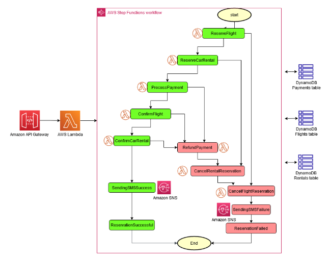
Workflow engines
A workflow engine stores workflow state durably, schedules activities, handles timers, retries failed steps, and resumes execution after worker crashes. This is different from a queue because the workflow engine remembers the logical process, not only the next message.
Temporal is a concrete workflow engine. Its documentation says a Workflow Execution is a durable, reliable, scalable function execution, and its platform material describes Activities as failure-prone functions that can retry automatically and recover from timeouts, API failures, and worker failures. Temporal Workflow Execution overview and Understanding Temporal are useful references for durable execution and activity retry behavior.
A durable workflow shape:
```python id=”durable-workflow-shape” @workflow def onboarding_workflow(user_id): profile = execute_activity(create_profile, user_id) billing = execute_activity(setup_billing, user_id) email = execute_activity(send_welcome_email, user_id)
return {
    "profile_id": profile.id,
    "billing_id": billing.id,
    "email_id": email.id,
} ```
The workflow engine records enough history to replay deterministic workflow code:
```python id=”workflow-history” [ {“event”: “WorkflowStarted”, “user_id”: “u123”}, {“event”: “ActivityScheduled”, “name”: “create_profile”}, {“event”: “ActivityCompleted”, “result”: {“profile_id”: “p456”}}, {“event”: “ActivityScheduled”, “name”: “setup_billing”}, {“event”: “ActivityFailed”, “reason”: “timeout”}, {“event”: “ActivityRetried”, “attempt”: 2} ]
A critical workflow-engine constraint is deterministic workflow code. If the workflow function calls random number generation, local wall-clock time, or external APIs directly during replay, it may diverge from its recorded history. External side effects should be activities, and nondeterministic results should be recorded in workflow history.

### Timers, retries, and durable waiting

Workflows often need to wait: wait for payment settlement, wait until tomorrow, wait for human approval, wait for a partner callback, or wait for a timeout. Durable timers allow the workflow to sleep without holding a worker thread or database transaction.

```python id="durable-timer"
@workflow
def subscription_trial(user_id):
    execute_activity(start_trial, user_id)

    workflow.sleep(days=14)

    if not execute_activity(has_user_cancelled, user_id):
        execute_activity(charge_subscription, user_id)
A queue can delay a message, but a workflow engine can represent the whole process and its history. The difference matters when there are multiple timers, branches, compensations, callbacks, and retries.
Try-confirm-cancel
Try-confirm-cancel, or TCC, is a business transaction pattern. Each participant exposes three operations:
| Operation | Meaning |
|---|---|
| Try | Reserve resources tentatively |
| Confirm | Make reservation permanent |
| Cancel | Release tentative reservation |
Example:
```python id=”tcc-interface” class InventoryService: def try_reserve(self, reservation_id, sku, quantity): …
def confirm_reservation(self, reservation_id):
    ...

def cancel_reservation(self, reservation_id):
    ... ```
TCC is useful when participants can hold a reservation with an expiration. It is common in booking, ticketing, inventory, payment authorization, quota allocation, and capacity management.
```python id=”tcc-checkout” def checkout(order_id): inventory.try_reserve(order_id, sku=”book-123”, quantity=1) payment.try_authorize(order_id, amount_cents=2500)
try:
    inventory.confirm_reservation(order_id)
    payment.confirm_authorization(order_id)
    orders.mark_confirmed(order_id)

except Exception:
    inventory.cancel_reservation(order_id)
    payment.cancel_authorization(order_id)
    orders.mark_failed(order_id) ```
TCC is not a substitute for every transaction. It requires participant APIs to support tentative state, expiration, confirmation, and cancellation. If a participant cannot reserve or compensate, TCC does not apply cleanly.
Human-in-the-loop workflows
Many production workflows include humans: fraud review, support approval, security access requests, legal review, data deletion approval, procurement, incident escalation, or model-evaluation review. These workflows cannot hold database locks while waiting for a person.
A human approval workflow:
```python id=”human-approval-workflow” @workflow def access_request_workflow(request_id): execute_activity(create_access_ticket, request_id)
approval = wait_for_signal(
    signal_name="approval_decision",
    timeout_days=7,
)

if approval == "approved":
    execute_activity(grant_access, request_id)
else:
    execute_activity(deny_access, request_id) ```
The distributed-systems issue is that a human response is another asynchronous message. It can arrive late, arrive twice, be edited, be revoked, or race with timeout. The workflow must record decision version, actor identity, timestamp, and authorization context.
```python id=”approval-signal-dedupe” def record_approval_signal(workflow_id, decision_id, actor, decision): with db.transaction() as tx: if tx.exists(“workflow_signals”, decision_id): return “duplicate”
    tx.insert("workflow_signals", {
        "decision_id": decision_id,
        "workflow_id": workflow_id,
        "actor": actor,
        "decision": decision,
    })

    tx.update("workflows", workflow_id, {
        "approval_state": decision,
        "approval_actor": actor,
    }) ```
Workflow state machines
Workflows should usually be explicit state machines. Implicit workflows hidden across logs and service side effects are hard to debug and recover.
```python id=”explicit-workflow-state” @dataclass class WorkflowState: workflow_id: str state: str version: int last_error: str | None updated_at_ms: int
VALID_TRANSITIONS = { “CREATED”: {“RESERVING_INVENTORY”, “CANCELLED”}, “RESERVING_INVENTORY”: {“AUTHORIZING_PAYMENT”, “COMPENSATING”}, “AUTHORIZING_PAYMENT”: {“CREATING_SHIPMENT”, “COMPENSATING”}, “CREATING_SHIPMENT”: {“CONFIRMED”, “COMPENSATING”}, “COMPENSATING”: {“FAILED”, “CANCELLED”}, }
Version-guarded transition:

```python id="workflow-state-transition"
def transition(workflow_id, expected_version, next_state):
    with db.transaction() as tx:
        state = tx.get("workflows", workflow_id)

        if state.version != expected_version:
            raise Conflict()

        if next_state not in VALID_TRANSITIONS[state.state]:
            raise InvalidTransition(state.state, next_state)

        state.state = next_state
        state.version += 1
        tx.put("workflows", workflow_id, state)
The version check prevents two workers from advancing the same workflow concurrently in incompatible ways.
Durable execution versus distributed transactions
Durable execution and distributed transactions solve different problems.
| Need | Better fit |
|---|---|
| Atomic update of several rows in one database | Local transaction |
| Atomic update across replicated ranges | Distributed transaction |
| Reserve, pay, ship, notify over minutes | Saga or workflow |
| Retry flaky API calls safely | Workflow with idempotent activities |
| Keep source DB and event stream aligned | Transactional outbox |
| Process Kafka input and produce Kafka output atomically | Kafka transaction |
| Enforce global uniqueness | Linearizable transaction or compare-and-swap |
| Coordinate human approval | Workflow engine |
| Undo business steps after partial failure | Saga compensation |
A practical rule:
\[\text{Use transactions for short atomic invariants; use workflows for long-running business processes.}\]Holding locks while waiting for a human, partner API, batch job, or warehouse action is usually the wrong design.
Exactly-once business effects
Exactly-once is often misunderstood. A system can provide exactly-once within a bounded domain, such as Kafka input offsets plus Kafka output records, or one database transaction. But end-to-end exactly-once across arbitrary APIs, emails, payments, queues, and databases is usually built from idempotency, deduplication, reconciliation, and atomic local boundaries.
Useful decomposition:
| Boundary | Mechanism |
|---|---|
| One database | Transaction |
| One Kafka read-process-write pipeline | Kafka transaction |
| DB plus outbound event | Transactional outbox |
| Inbound event plus DB effect | Inbox or processed-message table |
| External payment | Idempotency key at payment provider |
| Workflow activity | Activity ID and retry policy |
| Human decision | Decision ID and versioned state |
| Derived projection | Source offset stored with projection state |
A generic processed-effect table:
```sql id=”processed-effects-table” create table processed_effects ( effect_type text not null, idempotency_key text not null, result_json jsonb not null, created_at timestamp not null default current_timestamp, primary key (effect_type, idempotency_key) );
Handler:

```python id="processed-effect-wrapper"
def run_effect_once(effect_type, key, effect):
    with db.transaction() as tx:
        existing = tx.get("processed_effects", (effect_type, key))

        if existing:
            return existing.result_json

        result = effect()

        tx.insert("processed_effects", {
            "effect_type": effect_type,
            "idempotency_key": key,
            "result_json": result,
        })

        return result
This pattern works only if the effect itself can be made safe. If effect() calls an external service that does not support idempotency, the local database cannot guarantee the external service did not perform it twice.
Reconciliation
Reconciliation is the process of comparing actual state against expected state and repairing differences. It is not a failure of design. It is a normal part of distributed workflows where external systems, queues, retries, and partial failures exist.
Example: payment reconciliation.
```python id=”payment-reconciliation” def reconcile_payments(): pending = db.query(“”” select * from payments where status in (‘authorizing’, ‘unknown’) and updated_at < now() - interval ‘5 minutes’ “””)
for payment in pending:
    provider_status = payment_provider.get(payment.provider_id)

    if provider_status == "authorized":
        db.update("payments", payment.id, {"status": "authorized"})

    elif provider_status == "declined":
        db.update("payments", payment.id, {"status": "declined"})

    elif provider_status == "not_found":
        retry_or_mark_failed(payment) ```
Reconciliation should be designed into the workflow from the beginning. Every external side effect should have a stable identifier, a query API if possible, and a repair path.
Compensating transactions
A compensating transaction is a business operation that semantically counteracts a prior committed operation.
Examples:
| Original action | Compensation |
|---|---|
| Reserve inventory | Release reservation |
| Authorize payment | Void authorization |
| Capture payment | Refund payment |
| Create shipment | Cancel shipment if not shipped |
| Grant access | Revoke access |
| Send email | Send correction email |
| Create account | Disable account |
Compensation should be idempotent:
```python id=”idempotent-compensation” def release_inventory(reservation_id): with db.transaction() as tx: reservation = tx.get(“reservations”, reservation_id)
    if reservation.status == "released":
        return "already_released"

    if reservation.status == "confirmed":
        raise CannotReleaseConfirmedReservation()

    reservation.status = "released"
    tx.put("reservations", reservation_id, reservation)

    tx.increment("inventory", reservation.sku, reservation.quantity)

return "released" ```
Compensation should also be ordered in reverse dependency order. If shipment creation depends on payment authorization and inventory reservation, cancellation should usually cancel shipment first, then payment, then inventory.
Dead-letter queues and poison workflow steps
A poison message or poison workflow step repeatedly fails because the input is malformed, a dependency always rejects it, a schema changed incompatibly, or the handler has a deterministic bug. Retrying forever can block partitions and waste capacity.
A dead-letter strategy:
```python id=”dead-letter-queue” def handle_message_with_dlq(message): try: process(message) broker.ack(message)
except PermanentError as error:
    broker.publish("dead-letter", {
        "message": message,
        "error": str(error),
        "failed_at_ms": now_ms(),
    })
    broker.ack(message)

except RetryableError:
    if message.attempts >= MAX_ATTEMPTS:
        broker.publish("dead-letter", {
            "message": message,
            "error": "retry limit exceeded",
        })
        broker.ack(message)
    else:
        broker.nack(message, requeue=True) ```
A dead-letter queue needs ownership. Someone must inspect, fix, replay, or discard messages. A DLQ without alarms and runbooks is just delayed data loss.
Workflow observability
Transactions and workflows need different observability.
Transaction metrics:
| Metric | Meaning |
|---|---|
| Commit latency | How long commits take |
| Abort rate | Contention or validation failures |
| Lock wait time | Blocking and deadlock risk |
| Prepared transaction age | 2PC blocking risk |
| Participant count | Distributed transaction fanout |
| Retry count | OCC or serializable contention |
| Deadlock count | Locking pressure |
Workflow metrics:
| Metric | Meaning |
|---|---|
| Workflow age | Long-running or stuck workflows |
| State distribution | Backlog by workflow stage |
| Activity retry count | Flaky dependencies |
| Compensation rate | Business failure or downstream instability |
| Timer backlog | Scheduler or worker pressure |
| Signal age | Human or callback delay |
| DLQ count | Poison messages |
| Reconciliation fixes | Hidden inconsistency rate |
A workflow monitor:
```python id=”workflow-monitor” def monitor_workflows(): counts = db.query(“”” select state, count(*) as count, max(now() - updated_at) as oldest_age from workflows group by state “””)
for row in counts:
    metrics.gauge("workflow.count", row.count, tags={"state": row.state})
    metrics.gauge("workflow.oldest_age_seconds", row.oldest_age, tags={"state": row.state})

    if row.oldest_age > max_allowed_age(row.state):
        alert("workflow state stuck", state=row.state, age=row.oldest_age) ```
The concrete production lesson is that a workflow’s state is part of the product. Users do not care whether the payment worker, queue, or shipment service failed. They care whether their order is stuck, cancelled, confirmed, or refunded.
Transaction and workflow testing
Transactions should be tested with concurrency and failure injection. Workflows should be tested with retries, duplicate callbacks, out-of-order messages, timeouts, compensation failures, and replay.
Transaction test:
```python id=”transaction-concurrency-test” def test_no_negative_balance_under_concurrency(): account = create_account(balance=100)
run_concurrently([
    lambda: withdraw(account.id, 80),
    lambda: withdraw(account.id, 80),
])

final = get_account(account.id)

assert final.balance >= 0
assert count_successful_withdrawals(account.id) == 1 ```
Workflow test:
```python id=”workflow-failure-test” def test_checkout_compensates_when_shipping_fails(): order_id = create_order()
inject_failure("shipping.create", error=RetryableThenPermanentError())

result = run_checkout_saga(order_id)

assert result.state == "FAILED"
assert inventory.reservation(order_id).status == "released"
assert payment.authorization(order_id).status == "voided" ```
Replay test for durable workflows:
```python id=”workflow-replay-test” def test_workflow_replay_is_deterministic(): history = load_workflow_history(“checkout-123”) replay_result = workflow_engine.replay(checkout_workflow, history)
assert replay_result.matches_recorded_history() ```
The replay test catches accidental nondeterminism such as calling local time, random, or external APIs inside workflow logic.
Concrete design examples
E-commerce checkout
A typical checkout should not be one giant distributed transaction across order, inventory, payment, shipping, and email systems. A better design is a workflow or saga.
| Step | Mechanism |
|---|---|
| Create order record | Local DB transaction |
| Reserve inventory | Idempotent TCC try step |
| Authorize payment | Idempotent external API call |
| Create shipment | Idempotent activity |
| Confirm order | Local DB transaction |
| Publish events | Transactional outbox |
| Send email | At-least-once activity with email dedupe |
| Repair stuck orders | Reconciliation job |
Bank transfer
A bank transfer usually needs stronger transactional semantics than checkout.
| Case | Mechanism |
|---|---|
| Same account shard | Local serializable transaction |
| Different shards in same database | Distributed transaction |
| Different banks | Workflow with ledger entries, settlement, reconciliation |
| External payment rail | Idempotency keys, durable workflow, reconciliation |
The key distinction is that a ledger should not rely on compensation to “undo” money creation. It should write immutable entries and use reversing entries when corrections are needed.
```python id=”ledger-reversal” def reverse_ledger_entry(original_entry_id, reason): original = ledger.get(original_entry_id)
ledger.append({
    "entry_id": new_uuid(),
    "account_id": original.account_id,
    "amount": -original.amount,
    "currency": original.currency,
    "reverses": original_entry_id,
    "reason": reason,
}) ```
User signup with email uniqueness
A signup flow might use a strong uniqueness transaction for email, then a workflow for the rest.
```python id=”signup-unique-email” def create_user(email, profile): with db.transaction(isolation=”serializable”) as tx: if tx.exists(“email_index”, email): raise EmailAlreadyUsed()
user_id = new_uuid()
tx.insert("users", user_id, profile)
tx.insert("email_index", email, user_id)
tx.insert("outbox", {
"type": "UserCreated",
"user_id": user_id,
"email": email,
})
return user_id ```
After commit, a workflow can send verification email, provision resources, create analytics records, and retry safely.
Choosing the right mechanism
| Problem | Recommended mechanism |
|---|---|
| Update several rows in one database | Local transaction |
| Update rows across distributed ranges with strong invariant | Distributed transaction |
| Coordinate commit across multiple resource managers | 2PC or consensus-backed commit |
| Publish event after DB write | Transactional outbox |
| Consume event and update DB | Inbox or dedupe table |
| Long-running business process | Saga or workflow engine |
| External API with retry ambiguity | Idempotency key plus reconciliation |
| Reversible multi-step process | Saga with compensating transactions |
| Reservation-based process | Try-confirm-cancel |
| Numeric capacity constraint | Escrow or bounded counter |
| Kafka-to-Kafka stream processing | Kafka transactions |
| Human approval | Durable workflow with signals |
| Search or analytics projection | At-least-once events plus idempotent projection |
| Global uniqueness | Linearizable transaction or compare-and-swap |
Common transaction and workflow failure modes
| Failure mode | Cause | Safer design |
|---|---|---|
| Partial commit across services | Dual write or no atomic boundary | 2PC, distributed DB transaction, or outbox |
| Prepared transactions block forever | 2PC coordinator failure | Replicated coordinator, timeout runbook, consensus-backed commit |
| Duplicate payment | Retry after unknown outcome | Idempotency key at payment provider |
| Lost event | DB commit succeeds but publish fails | Transactional outbox |
| Duplicate event effect | At-least-once delivery without dedupe | Inbox or processed-message table |
| Workflow stuck | Missing callback, worker failure, unhandled state | Durable workflow state and stuck-state alerts |
| Compensation fails | External system rejects undo | Idempotent compensation and reconciliation |
| Email sent twice | Activity retried without dedupe | Message ID or idempotency key |
| Write skew | Snapshot isolation with cross-row invariant | Serializable isolation or materialized constraint |
| Retry storm | All workflow activities retry aggressively | Backoff, jitter, retry budgets |
| DLQ ignored | Poison messages accumulate silently | Ownership, alerting, replay tooling |
| Non-deterministic workflow replay | Workflow code calls time, random, or external API | Record nondeterminism through workflow history |
| Cross-shard transaction too slow | Poor shard key or high participant count | Shard by transactional boundary or use saga |
| Outbox relay publishes twice | Crash after publish before marking sent | Consumer idempotency |
Deployment checklist for transactions and workflows
- Define the invariant: Know what must never happen before choosing a mechanism.
- Prefer local transactions: Shard so common invariants fit inside one partition.
- Use distributed transactions selectively: They are appropriate for strong atomicity, but they add coordination and recovery complexity.
- Make transaction retries safe: Serializable and OCC systems may abort valid concurrent work.
- Track prepared transaction age: Prepared 2PC participants are operationally dangerous if they linger.
- Avoid dual writes: Use outbox, CDC, or a real distributed transaction.
- Make consumers idempotent: At-least-once delivery is the normal case.
- Use stable operation IDs: Every external side effect should have a durable idempotency key.
- Distinguish rollback from compensation: Compensation is a new business action, not time travel.
- Model workflows explicitly: Store state, version, attempts, errors, and timestamps.
- Use durable timers: Do not hold locks or threads while waiting.
- Design reconciliation: External systems need query and repair paths.
- Observe workflow state: Monitor stuck workflows, retries, compensation rate, and DLQs.
- Test failure paths: Crash after prepare, after publish, before ack, after external side effect, and during compensation.
- Document exactly-once boundaries: Say exactly which system boundary provides atomicity, and where idempotency is required.
Transactions and workflows are the machinery that turns distributed storage and messaging into correct business behavior. Use transactions when the system needs a short atomic change over well-defined data. Use distributed transactions when a strong invariant truly spans partitions. Use outbox and inbox patterns when services communicate through events. Use sagas and workflow engines when the process is long-running, failure-prone, or involves external systems. Use idempotency and reconciliation everywhere side effects can be retried after an unknown outcome.
Distributed Compute
What distributed compute is
Distributed compute is the layer that splits work across many machines, schedules that work, moves data to the right place, retries failed tasks, aggregates results, and exposes a programming model that hides some of the underlying cluster complexity. Distributed storage answers “where does data live?” Distributed compute answers “where should work run, how should it be parallelized, and how should failures be recovered?”
A distributed compute system usually manages:
| Concern | What it means |
|---|---|
| Task decomposition | Split a job into independent or dependent units of work |
| Scheduling | Place tasks on machines with enough CPU, memory, disk, GPU, locality, and quota |
| Data movement | Move, shuffle, broadcast, cache, or colocate data |
| Fault tolerance | Retry failed tasks, recover lost intermediate state, or replay lineage |
| Progress tracking | Know which tasks are pending, running, failed, retried, or complete |
| Straggler handling | Reduce tail latency from unusually slow workers |
| Resource isolation | Prevent one job, tenant, or user from starving others |
| Backpressure | Slow producers when consumers, queues, or workers are saturated |
| Checkpointing | Save intermediate state so work can resume after failure |
| Output commit | Make final results visible exactly once or at least safely |
The simplest distributed compute model is embarrassingly parallel: split independent work items across workers and collect results. The hard cases involve dependencies, shuffles, stateful streaming, exactly-once output, GPU collectives, large intermediate data, heterogeneous resources, and failures that happen mid-computation. MapReduce: Simplified Data Processing on Large Clusters by Dean et al. (2004) is the classic production paper because it made large-scale batch computation usable by forcing programmers into map and reduce functions while the runtime handled partitioning, scheduling, locality, retry, and shuffle.
A useful compute-system lower bound is:
\[T_{\text{job}} \geq \max\left(\frac{W}{C},\ T_{\text{critical path}},\ T_{\text{data movement}}\right),\]where \(W\) is total work, \(C\) is available cluster capacity, \(T_{\text{critical path}}\) is the longest dependency chain, and \(T_{\text{data movement}}\) is time spent moving data. Adding machines helps only if the job has enough parallel work and data movement does not dominate.
Amdahl’s Law gives the same warning:
\[S(N) = \frac{1}{(1 - p) + \frac{p}{N}},\]where \(p\) is the parallelizable fraction and \(N\) is the number of workers. If a job has a large serial planning, shuffle, checkpoint, or output-commit phase, more machines will not produce linear speedup.
The compute model spectrum
Distributed compute systems differ by duration, dependency structure, state, and latency target.
| Model | Work unit | State model | Latency target | Concrete systems |
|---|---|---|---|---|
| Batch processing | Finite dataset and finite job | Usually bounded intermediate state | Minutes to hours | MapReduce, Hadoop, Spark, AWS Batch |
| DAG orchestration | Tasks connected by dependencies | Externalized task outputs | Minutes to days | Airflow, Argo Workflows, Step Functions |
| Stream processing | Unbounded event stream | Long-lived keyed state | Milliseconds to seconds | Flink, Kafka Streams, Beam/Dataflow, Samza |
| Dynamic task graphs | Fine-grained tasks with runtime dependencies | Objects, futures, actors | Milliseconds to minutes | Ray, Dask |
| Actor systems | Long-lived stateful processes | In-actor state | Low-latency interactions | Akka, Orleans, Ray actors |
| Serverless functions | Event-triggered functions | Mostly externalized state | Milliseconds to minutes | AWS Lambda, Cloud Functions |
| Distributed ML training | Gradients, tensors, optimizer state | Model, gradients, activations, optimizer state | Iterative training steps | Parameter servers, PyTorch Distributed, Megatron-LM, DeepSpeed, GShard |
| GPU inference serving | Requests, batches, sequences, KV cache | Model weights and request state | Milliseconds to seconds | Triton, Ray Serve, custom Kubernetes GPU fleets |
The right compute model depends on whether the workload is finite or unbounded, stateless or stateful, latency-sensitive or throughput-oriented, CPU-bound or I/O-bound, and whether correctness depends on exactly-once output, deterministic replay, or idempotent retries.
Batch processing
Batch processing runs a finite computation over a finite input. Inputs are usually files, object-store prefixes, tables, partitions, or snapshots. Outputs are usually new files, tables, indexes, reports, model artifacts, or materialized views. Batch jobs are easier than streaming jobs because the input has a known boundary, but they still need scheduling, shuffling, retries, output commits, and resource isolation.
Canonical examples:
| System | Concrete role |
|---|---|
| Google MapReduce | Large-scale internal batch processing over GFS |
| Hadoop MapReduce | Open-source MapReduce-style batch processing over HDFS |
| Apache Spark | In-memory batch and iterative processing using RDDs and DataFrames |
| AWS Batch | Managed batch scheduler that maps job queues to compute environments |
| Kubernetes Jobs | Cluster-native finite jobs with completions, parallelism, and indexed jobs |
| Argo Workflows | Container-native DAG and step workflows on Kubernetes |
AWS Batch compute environments explains a concrete managed-cloud batch design: job queues are mapped to one or more compute environments, and compute environments contain the container instances used to run jobs. Jobs explains the Kubernetes version: a Job creates Pods until a specified number of completions succeeds, and indexed Jobs give each Pod a stable completion index for partitioned work.
A generic batch job has this shape:
```python id=”batch-job-skeleton” def run_batch_job(input_partitions): task_ids = []
for partition in input_partitions:
task_id = scheduler.submit(
task_type="ProcessPartition",
payload={"partition": partition},
resources={"cpu": 2, "memory_gb": 8},
)
task_ids.append(task_id)
wait_for_all_success(task_ids)
scheduler.submit(
task_type="CommitOutput",
payload={"inputs": task_ids},
resources={"cpu": 1, "memory_gb": 4},
) ```
The important implementation detail is that each partition task should be idempotent. A worker can crash after writing partial output. The scheduler can retry the task. The output commit protocol must ensure only one successful attempt becomes visible.
```python id=”idempotent-batch-output” def process_partition(job_id, partition_id, attempt_id): temp_path = f”s3://bucket/jobs/{job_id}/tmp/{partition_id}/{attempt_id}/” final_path = f”s3://bucket/jobs/{job_id}/output/{partition_id}/”
rows = read_partition(partition_id)
output = transform(rows)
write_output(temp_path, output)
# Commit by atomically recording the winning attempt.
committed = commit_store.compare_and_swap(
key=f"{job_id}:{partition_id}",
expected=None,
value={"attempt_id": attempt_id, "path": temp_path},
)
if committed:
publish_manifest_entry(final_path, temp_path)
else:
cleanup_later(temp_path) ```
MapReduce
MapReduce decomposes a batch job into map tasks, shuffle, and reduce tasks. The user provides:
\[map(k_1, v_1) \rightarrow list(k_2, v_2)\] \[reduce(k_2, list(v_2)) \rightarrow list(v_3)\]The runtime partitions intermediate keys so that all values for the same key arrive at the same reducer. The MapReduce paper’s key production contribution is not the map and reduce functions alone, but the runtime around them: input splitting, task scheduling near data, intermediate data partitioning, retry after worker failure, backup tasks for stragglers, and atomic output handling. MapReduce: Simplified Data Processing on Large Clusters by Dean et al. (2004) is relevant here because it gives the execution model and the failure-handling mechanics that shaped later batch systems.
The following figure (source) shows the overview of the execution of a MapReduce operation, where input splits are processed by map workers, intermediate key ranges are shuffled to reduce workers, and final outputs are written to distributed storage.
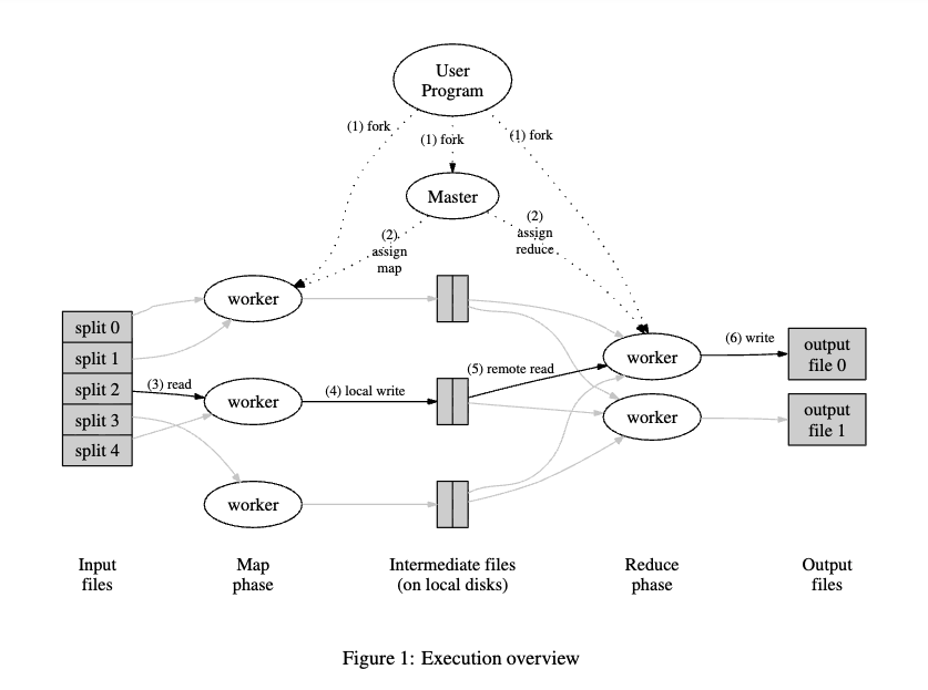
A word-count example:
```python id=”mapreduce-word-count” def map_fn(_file_name, line): for word in tokenize(line): emit(word, 1)
def reduce_fn(word, counts): emit(word, sum(counts))
A simplified MapReduce scheduler:
```python id="mapreduce-scheduler"
class MapReduceScheduler:
def run(self, input_splits, num_reducers):
map_tasks = [
self.submit_map(split, num_reducers)
for split in input_splits
]
self.wait_for_all(map_tasks)
reduce_tasks = [
self.submit_reduce(reducer_id)
for reducer_id in range(num_reducers)
]
self.wait_for_all(reduce_tasks)
self.commit_job_output()
The shuffle is the expensive part. Every mapper writes intermediate records partitioned by reducer:
```python id=”mapreduce-shuffle-partition” def partition_intermediate_key(key, num_reducers): return stable_hash(key) % num_reducers
If there are $$M$$ map tasks and $$R$$ reduce tasks, the shuffle can create up to:
$$
M \times R
$$
intermediate partitions. Large shuffles stress disk, network, file metadata, serialization, compression, and reducer skew. This is why production MapReduce-style systems spend significant engineering effort on combiners, compression, partitioning, skew handling, locality, and speculative execution.
### Stragglers and speculative execution
A straggler is a task that runs much slower than other equivalent tasks. Causes include slow disks, noisy neighbors, bad input split, GC pauses, network congestion, degraded hardware, or skewed keys. In a job with many parallel tasks, the job finishes when the slowest required task finishes:
$$
T_{\text{stage}} = \max_{i=1}^{n} T_i.
$$
Even rare slow tasks can dominate tail latency. The MapReduce paper describes backup task execution near the end of a job: the master schedules duplicate executions of remaining in-progress tasks, and the job uses whichever attempt finishes first.
A speculative execution sketch:
```python id="speculative-execution"
def maybe_launch_speculative_attempt(task):
if task.progress_percent < expected_progress(task.runtime_seconds):
if not task.has_speculative_attempt:
scheduler.submit(
task_type=task.task_type,
payload=task.payload,
attempt_type="speculative",
)
task.has_speculative_attempt = True
Speculation is safe only if tasks are idempotent and output commit handles duplicate attempts. It is helpful for read-only map tasks, deterministic transforms, and pure computations. It is dangerous for non-idempotent external effects.
Spark and lineage-based recovery
Spark generalized batch compute beyond MapReduce by representing computations as DAGs over resilient distributed datasets, or RDDs. Resilient Distributed Datasets: A Fault-Tolerant Abstraction for In-Memory Cluster Computing by Zaharia et al. (2012) introduced RDDs as immutable, partitioned collections that can be rebuilt from lineage after failure, which makes them efficient for iterative algorithms and interactive data mining where intermediate data is reused in memory.
The following figure (source) shows RDD lineage, where derived datasets remember the transformations needed to reconstruct lost partitions rather than replicating every intermediate result eagerly.
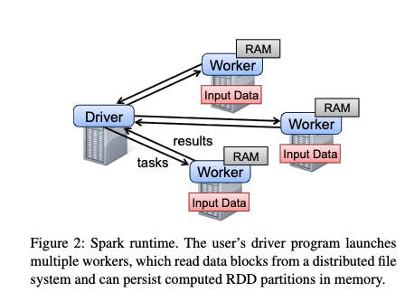
A Spark-like computation:
```python id=”spark-like-rdd” logs = read_text(“s3://logs/2026-07-04/”) errors = logs.filter(lambda line: “ERROR” in line) pairs = errors.map(lambda line: (extract_service(line), 1)) counts = pairs.reduce_by_key(lambda a, b: a + b)
counts.write(“s3://reports/errors-by-service/”)
The compute DAG has narrow and wide dependencies. A narrow dependency means one output partition depends on a small number of input partitions, often one. A wide dependency means output requires data from many input partitions, usually through shuffle.
```python id="narrow-vs-wide-dependency"
# Narrow dependency: partition i can be computed from partition i.
filtered = logs.filter(is_error)
# Wide dependency: records must be repartitioned by key across the cluster.
counts = filtered.map(to_service_pair).reduce_by_key(sum_values)
Spark’s lineage model means lost partitions can be recomputed:
```python id=”lineage-recompute” def compute_partition(rdd, partition_id): if cache.contains(rdd.id, partition_id): return cache.get(rdd.id, partition_id)
parent_results = [
compute_partition(parent_rdd, parent_partition)
for parent_rdd, parent_partition in rdd.dependencies(partition_id)
]
result = rdd.compute(parent_results)
cache.put(rdd.id, partition_id, result)
return result ```
Lineage is excellent for deterministic recomputation. It is less suitable when tasks perform external side effects, use nondeterministic code, or depend on data that has changed since the original computation.
Shuffles
A shuffle redistributes data across workers, usually by key. Shuffles are necessary for group-by, reduce-by-key, joins, repartitions, sorts, and aggregations. They are expensive because they combine network I/O, disk spill, memory pressure, serialization, and synchronization between stages.
Shuffle volume can be approximated as:
\[V_{\text{shuffle}} = \sum_{r \in records} size(r).\]If each record is copied once across the network, network time is bounded by:
\[T_{\text{shuffle}} \geq \frac{V_{\text{shuffle}}}{B_{\text{network}}}.\]This lower bound ignores serialization, disk spill, compression, retries, skew, and connection overhead.
A local combiner can reduce shuffle volume:
```python id=”local-combiner” def map_partition(records): local_counts = {}
for record in records:
key = extract_key(record)
local_counts[key] = local_counts.get(key, 0) + 1
for key, count in local_counts.items():
emit(key, count) ```
A skewed key can overload one reducer:
```python id=”skewed-key”
Bad if one customer_id dominates the dataset.
partition = stable_hash(customer_id) % num_reducers
A salted-key mitigation:
```python id="salted-key-aggregation"
def salted_key(key, salt_count):
salt = random_int(0, salt_count - 1)
return (key, salt)
# First aggregate by salted key, then merge the partials by original key.
Real systems such as Spark and Flink include shuffle managers, sorters, spill files, compression, and adaptive execution strategies because shuffle is often the dominant cost of large data jobs.
Batch scheduling
A batch scheduler decides which task runs where and when. It must respect dependencies, resource requests, priorities, quotas, locality, retries, and preemption. A simple scheduler loop:
```python id=”batch-scheduler-loop” def scheduler_loop(): while True: runnable = find_tasks_whose_dependencies_succeeded() available_workers = find_workers_with_free_resources()
for task in prioritize(runnable):
worker = choose_worker(task, available_workers)
if worker is None:
continue
assign(task, worker)
reserve_resources(worker, task.resources)
sleep(SCHEDULER_INTERVAL) ```
A placement function:
```python id=”task-placement” def choose_worker(task, workers): candidates = [ worker for worker in workers if worker.free_cpu >= task.cpu and worker.free_memory_gb >= task.memory_gb and task.required_gpu_type in worker.gpu_types ]
if task.input_location:
candidates = sort_by_data_locality(candidates, task.input_location)
return least_loaded(candidates) ```
AWS Batch gives a managed version of this: users submit jobs into job queues, queues map to compute environments, and the scheduler chooses compute environments according to queue configuration and order. Kubernetes Jobs give a lower-level cluster-native version where the Kubernetes controller creates Pods until the desired number of completions succeeds.
A Kubernetes indexed Job example:
```yaml id=”kubernetes-indexed-job” apiVersion: batch/v1 kind: Job metadata: name: partitioned-backfill spec: completions: 1000 parallelism: 50 completionMode: Indexed template: spec: restartPolicy: Never containers: - name: worker image: example/backfill:2026-07-04 env: - name: PARTITION_INDEX valueFrom: fieldRef: fieldPath: metadata.annotations[‘batch.kubernetes.io/job-completion-index’]
This is a concrete deployment pattern for partitioned backfills: each Pod gets a stable index, processes one partition, writes idempotent output, and exits.
### DAG orchestration
A DAG orchestrator runs tasks with dependencies. It is used for ETL, data pipelines, backfills, feature generation, reporting, model training workflows, and operational workflows. The DAG itself is not the compute engine for every task. It is often the coordinator that starts Spark jobs, SQL queries, container jobs, Kubernetes Jobs, Lambda functions, or external service calls.
Airflow is a common example. [Dags](https://airflow.apache.org/docs/apache-airflow/stable/core-concepts/dags.html) explains that Airflow loads DAGs from Python source files, and [Apache Airflow](https://airflow.apache.org/) describes Airflow as a platform to programmatically author, schedule, and monitor workflows. Argo Workflows is the Kubernetes-native version; its [DAG](https://argo-workflows.readthedocs.io/en/latest/walk-through/dag/) documentation says DAGs specify task dependencies and allow maximum parallelism once dependencies are satisfied.
An Airflow-style DAG:
```python id="airflow-dag-example"
from airflow import DAG
from airflow.operators.bash import BashOperator
with DAG(
dag_id="daily_feature_pipeline",
schedule="@daily",
catchup=True,
) as dag:
extract = BashOperator(
task_id="extract",
bash_command="python extract.py --date ",
)
transform = BashOperator(
task_id="transform",
bash_command="spark-submit transform.py --date ",
)
validate = BashOperator(
task_id="validate",
bash_command="python validate.py --date ",
)
publish = BashOperator(
task_id="publish",
bash_command="python publish.py --date ",
)
extract >> transform >> validate >> publish
An Argo DAG:
```yaml id=”argo-dag-example” apiVersion: argoproj.io/v1alpha1 kind: Workflow metadata: generateName: daily-feature-pipeline- spec: entrypoint: pipeline templates: - name: pipeline dag: tasks: - name: extract template: run arguments: parameters: - name: command value: “python extract.py”
- name: transform
template: run
dependencies: [extract]
arguments:
parameters:
- name: command
value: "spark-submit transform.py"
- name: validate
template: run
dependencies: [transform]
arguments:
parameters:
- name: command
value: "python validate.py"
- name: run
inputs:
parameters:
- name: command
container:
image: example/pipeline:latest
command: ["sh", "-c"]
args: [""] ```
A DAG scheduler must handle retries and idempotency. If publish fails and reruns, it should not publish two conflicting versions. A robust DAG task writes to a temporary location and commits with a manifest or version pointer.
Workflow DAGs versus dataflow DAGs
DAG orchestration and dataflow execution are related but different.
| Aspect | Workflow DAG | Dataflow DAG |
|---|---|---|
| Node | Task, job, container, SQL query, API call | Operator, transformation, stage |
| Edge | Dependency or artifact | Data stream or partition dependency |
| Scheduler | Airflow, Argo, Step Functions | Spark, Flink, Beam runner |
| State | Usually externalized in storage | Runtime-managed partitions or keyed state |
| Failure recovery | Retry task or resume workflow | Recompute lineage, restore checkpoint, replay stream |
| Latency | Often minutes or longer | Batch seconds to hours, streaming milliseconds to seconds |
A workflow DAG might launch a Spark job. Inside that Spark job, Spark builds its own dataflow DAG. Mixing these up leads to bad designs: Airflow should not orchestrate millions of per-record tasks, and Spark should not coordinate human approval workflows.
Stream processing
Stream processing runs continuous computations over unbounded input. The input may be Kafka topics, Kinesis streams, Pub/Sub subscriptions, change streams, logs, metrics, clicks, payments, IoT events, or CDC records. Stream processors usually provide event-time processing, windowing, keyed state, checkpoints, and exactly-once or at-least-once semantics within a defined boundary.
The Dataflow Model: A Practical Approach to Balancing Correctness, Latency, and Cost in Massive-Scale, Unbounded, Out-of-Order Data Processing by Akidau et al. (2015) is central because it separates event time from processing time, formalizes windows, triggers, watermarks, and accumulation, and explains how modern systems balance correctness, latency, and cost for out-of-order unbounded data. Apache Beam Programming Guide gives the concrete programming model around windows, watermarks, and triggers.
The following figure (source) shows the Dataflow model’s distinction between event time and processing time, illustrating why unbounded out-of-order streams require watermarks, windows, and triggers rather than simple arrival-time batching.

Event time is when the event actually happened:
\[t_{\text{event}}.\]Processing time is when the system observes or processes the event:
\[t_{\text{processing}}.\]A late event has:
\[t_{\text{processing}} \gg t_{\text{event}}.\]A streaming word count by fixed event-time window:
```python id=”streaming-windowed-count” def process_event(event): window_start = floor_to_minute(event.event_time) window_end = window_start + 60
key = (event.word, window_start, window_end)
state[key] = state.get(key, 0) + 1
def on_watermark(watermark_time): for (word, start, end), count in state.items(): if end <= watermark_time: emit({ “word”: word, “window_start”: start, “window_end”: end, “count”: count, }) delete_state((word, start, end))
This sketch is incomplete because real systems must handle late data, triggers, accumulation modes, state TTL, checkpointing, and output idempotency.
### Watermarks, windows, and triggers
A watermark is the system’s estimate that it has likely seen all events earlier than some event time. Apache Beam describes watermarks as the system’s notion of input completeness for a pipeline, and Beam triggers can emit early results before a window is complete or late results after the watermark passes the end of a window.
A window assignment:
$$
window(t) = \left[\left\lfloor \frac{t}{W} \right\rfloor W,\ \left(\left\lfloor \frac{t}{W} \right\rfloor + 1\right)W\right)
$$
where $$W$$ is the window size.
Trigger choices:
| Trigger | Purpose |
| ----------------------- | ------------------------------------- |
| Event-time trigger | Emit when watermark passes window end |
| Processing-time trigger | Emit after wall-clock delay |
| Count trigger | Emit after enough events arrive |
| Early trigger | Emit low-latency partial result |
| Late trigger | Revise result after late data |
A stream processor must choose accumulation behavior:
| Mode | Meaning |
| --------------------------- | ------------------------------------------------------ |
| Discarding | Each pane contains only new data since prior firing |
| Accumulating | Each pane contains all data seen so far for the window |
| Accumulating and retracting | Later panes correct prior outputs |
This matters for downstream consumers. If a dashboard expects replacement results but the stream emits deltas, counts will be wrong.
### Stateful stream processing
Stateful stream processing stores per-key state across events: counts, sessions, joins, dedupe sets, windows, fraud scores, user profiles, or partial aggregates. Apache Flink describes itself as a framework for stateful computations over bounded and unbounded streams, and its stateful stream processing documentation says a streaming dataflow can be resumed from a checkpoint while maintaining exactly-once processing semantics. Kafka Streams also exposes fault-tolerant local state and exactly-once processing semantics within Kafka.
A keyed dedupe operator:
```python id="stream-deduplication"
def process_event(event):
key = event.event_id
if state.contains(key):
return
state.put(key, True, ttl_hours=24)
emit(event)
A sessionization operator:
```python id=”stream-sessionization” SESSION_GAP_SECONDS = 30 * 60
def process_click(event): session = state.get(event.user_id)
if session is None or event.event_time - session.last_seen > SESSION_GAP_SECONDS:
session = {
"session_id": new_session_id(),
"user_id": event.user_id,
"start_time": event.event_time,
"events": [],
}
session["events"].append(event)
session["last_seen"] = event.event_time
state.put(event.user_id, session) ```
The state store must be checkpointed or replicated. If a worker fails and loses local state, the processor must restore from a checkpoint or replay the source stream from a known offset.
Checkpointing in streams
Checkpointing captures operator state and input positions so a streaming job can recover consistently. Flink’s checkpointing documentation says exactly-once is preferable for most applications, and its stateful processing page says stream dataflows can resume from checkpoints while maintaining consistency. Lightweight Asynchronous Snapshots for Distributed Dataflows by Carbone et al. (2015) describes asynchronous barrier snapshotting, a checkpointing algorithm implemented in Apache Flink that avoids stopping the whole stream topology.
The following figure (source) shows asynchronous barrier snapshotting, where checkpoint barriers flow through the dataflow graph and separate records before and after a snapshot without stopping ordinary stream processing.

A checkpoint record usually includes:
| Component | Example |
|---|---|
| Source offsets | Kafka topic, partition, offset |
| Operator state | RocksDB state, window state, timers |
| In-flight barriers | Barrier alignment state |
| Sink transaction handles | Pending output transactions |
| Job graph version | Operator IDs and topology |
A simplified checkpoint:
```python id=”stream-checkpoint” def take_checkpoint(checkpoint_id): pause_or_align_inputs(checkpoint_id)
snapshot = {
"checkpoint_id": checkpoint_id,
"source_offsets": source.current_offsets(),
"operator_state": state_backend.snapshot(),
"timers": timer_service.snapshot(),
}
durable_store.write(
path=f"checkpoints/{checkpoint_id}/metadata.json",
value=json_encode(snapshot),
)
acknowledge_checkpoint(checkpoint_id) ```
Recovery:
```python id=”stream-recovery” def recover_from_checkpoint(checkpoint_id): snapshot = durable_store.read(f”checkpoints/{checkpoint_id}/metadata.json”)
source.seek(snapshot["source_offsets"])
state_backend.restore(snapshot["operator_state"])
timer_service.restore(snapshot["timers"])
start_processing() ```
Exactly-once output requires the sink to participate. A stream processor can restore source offsets and state exactly, but if the sink wrote external records before failure without an atomic commit protocol, downstream effects may duplicate. This is why Kafka-to-Kafka exactly-once is easier than Kafka-to-email or Kafka-to-payment exactly-once.
Kafka Streams, Flink, and Beam in practice
Concrete stream systems make different tradeoffs:
| System | Practical fit | Key mechanics |
|---|---|---|
| Kafka Streams | Application library for Kafka-native stream processing | Topic partitions, local state stores, changelog topics, Kafka transactions |
| Flink | General-purpose stateful stream and batch engine | Checkpoints, watermarks, keyed state, event time, savepoints |
| Beam/Dataflow | Portable programming model and managed runner option | Windows, triggers, watermarks, runners |
| Samza | Stream processing with local state, historically LinkedIn/Kafka-oriented | Partitioned local state and changelogs |
| Spark Structured Streaming | Streaming model integrated with Spark SQL/DataFrames | Micro-batches or continuous execution, checkpoints |
Kafka Streams’ concrete deployment advantage is operational locality: a stream application is just a client application consuming and producing Kafka topics, with local state backed by changelog topics. Flink’s advantage is richer long-running stateful processing with checkpointing and event-time semantics. Beam’s advantage is a programming model that can target different runners, with Google Cloud Dataflow as the managed Google runner.
Dynamic task graphs: Ray and Dask
Some workloads need more dynamic task graphs than traditional batch DAGs. Reinforcement learning, hyperparameter search, simulation, distributed Python, model serving, and mixed training-serving loops often create tasks at runtime and need futures, actors, and object stores.
Ray: A Distributed Framework for Emerging AI Applications by Moritz et al. (2018) presents Ray as a cluster-computing framework with a unified interface for task-parallel and actor-based computations, backed by a dynamic execution engine. Dask.distributed describes Dask’s distributed scheduler as a centrally managed dynamic task scheduler coordinating workers and clients across machines.
The following figure (source) shows Ray’s system architecture, where a global control store, distributed scheduler, workers, and object store support both tasks and actors.

A Ray-style task API:
```python id=”ray-style-task” @remote def score_model(config): model = train(config) return evaluate(model)
futures = [ score_model.remote(config) for config in hyperparameter_configs ]
scores = ray.get(futures)
An actor-style API:
```python id="ray-style-actor"
@remote
class ParameterActor:
def __init__(self):
self.weights = initialize_weights()
def get_weights(self):
return self.weights
def apply_gradient(self, gradient):
self.weights = update(self.weights, gradient)
return self.weights
parameter_actor = ParameterActor.remote()
Dynamic task systems need object management. Passing large values by value can crush the scheduler and network. A better design stores large objects in a distributed object store and passes references.
```python id=”pass-by-reference” dataset_ref = object_store.put(large_dataset)
futures = [ train_partition.remote(dataset_ref, partition_id) for partition_id in range(1000) ]
### Actor systems
The actor model represents computation as independent stateful actors that communicate through messages. Each actor owns its state and processes messages, usually one at a time. This avoids shared-memory locking inside the actor, but introduces distributed messaging, placement, supervision, and state recovery problems.
Actor model:
$$
actor = (state,\ mailbox,\ behavior)
$$
On message:
$$
(state', outgoing) = behavior(state,\ message)
$$
A simple actor:
```python id="actor-counter"
class CounterActor:
def __init__(self):
self.count = 0
def on_message(self, message):
if message["type"] == "increment":
self.count += message["amount"]
return {"count": self.count}
if message["type"] == "get":
return {"count": self.count}
Actors are useful for stateful services, game sessions, real-time coordination, simulations, user sessions, workflow entities, and ML serving state. The hard deployment questions are:
| Question | Why it matters |
|---|---|
| Where is the actor placed? | Latency, locality, and load |
| How is actor state recovered? | Worker crash should not lose durable state |
| Are messages ordered? | Per-sender and per-actor ordering affect correctness |
| Are messages deduplicated? | Retries can duplicate side effects |
| Can actors move? | Rebalancing and failure recovery |
| What happens to long mailboxes? | Backpressure and memory safety |
A durable actor writes events or snapshots:
```python id=”durable-actor” class DurableCounterActor: def init(self, actor_id): self.actor_id = actor_id self.count = load_snapshot(actor_id)
def increment(self, command_id, amount):
if already_processed(command_id):
return self.count
event_log.append({
"actor_id": self.actor_id,
"command_id": command_id,
"type": "Incremented",
"amount": amount,
})
self.count += amount
mark_processed(command_id)
return self.count ```
This is the same theme as the rest of distributed systems: retries require idempotency, and local state needs a durable recovery anchor.
Serverless compute
Serverless functions execute code in response to events without the user managing servers directly. The platform handles provisioning, scaling, placement, isolation, and lifecycle. The application must still handle idempotency, timeouts, cold starts, concurrency, retries, and externalized state.
AWS Lambda is the canonical managed example. Understanding Lambda function scaling says Lambda scales execution environment instances as a function receives more concurrent requests. How Lambda processes records from stream and queue-based event sources says event source mappings read from streams and queues and invoke Lambda functions with batches of records.
A Lambda-style handler must be idempotent:
```python id=”lambda-idempotent-handler” def handler(event, context): for record in event[“Records”]: message_id = record[“messageId”]
with db.transaction() as tx:
if tx.exists("processed_messages", message_id):
continue
process_record(tx, record)
tx.insert("processed_messages", {
"message_id": message_id,
"processed_at": now_ms(),
})
return {"status": "ok"} ```
Serverless queue processing introduces a batch boundary. If one record in the batch fails, the platform may retry the batch or partial batch depending on configuration. The handler should either support per-record failure reporting or make every record idempotent.
Serverless is good for bursty event-driven compute, glue logic, webhooks, lightweight transformations, scheduled jobs, and asynchronous integration. It is less natural for long-running jobs, tightly coupled distributed training, large local state, low-latency warm connections, or workloads requiring precise placement.
Compute placement and data locality
Data locality reduces data movement by scheduling work near input data. This was central to GFS plus MapReduce, where map tasks were scheduled near chunk replicas. In object-store-based cloud systems, locality is less explicit but still matters through region, availability zone, network path, cache, and data format.
A locality-aware scheduler:
```python id=”data-locality-scheduler” def choose_worker_for_split(split, workers): preferred_nodes = storage.locations_for_split(split)
local_candidates = [
worker for worker in workers
if worker.node_id in preferred_nodes and worker.has_capacity()
]
if local_candidates:
return least_loaded(local_candidates)
return least_loaded([worker for worker in workers if worker.has_capacity()]) ```
Data locality tradeoff:
| Choice | Benefit | Cost |
|---|---|---|
| Wait for local worker | Less network I/O | Higher queueing delay |
| Run immediately elsewhere | Lower scheduling delay | More network I/O |
| Cache reused data | Faster iterative jobs | Memory pressure |
| Broadcast small data | Avoid repeated lookups | Driver and network pressure |
| Shuffle large data | General joins and aggregations | Expensive network and disk |
Spark’s RDD paper is relevant because RDDs let iterative jobs reuse working sets in memory while retaining fault tolerance through lineage, which directly targets workloads where repeated disk I/O dominates runtime.
Output commit protocols
Distributed compute jobs often produce many output files or partitions. A job should make outputs visible atomically enough that readers do not see partial results. This is usually done with temporary paths plus a manifest, version pointer, or transactional table commit.
Bad pattern:
```python id=”bad-output-commit” def write_partition(partition_id, rows): path = f”s3://reports/current/part-{partition_id}.parquet” write_file(path, rows)
If the job fails halfway, readers may see a mix of old and new output.
Safer pattern:
```python id="manifest-output-commit"
def write_job_output(job_id, partitions):
temp_prefix = f"s3://reports/tmp/{job_id}/"
final_manifest = f"s3://reports/manifests/{job_id}.json"
files = []
for partition_id, rows in partitions:
path = f"{temp_prefix}/part-{partition_id}.parquet"
write_file(path, rows)
files.append(path)
manifest = {
"job_id": job_id,
"files": files,
"created_at_ms": now_ms(),
}
write_file(final_manifest, json_encode(manifest))
# Commit point: update small pointer after all files exist.
write_file("s3://reports/current_manifest.json", json_encode({
"manifest": final_manifest,
}))
The invariant is:
\[\text{readers use only committed manifests, never partial directory contents}.\]This pattern appears in data lake table formats, checkpointed ML artifacts, batch outputs, and backfills.
Backfills
A backfill recomputes historical data. Backfills are operationally risky because they can create massive load on storage, queues, databases, caches, and downstream consumers.
A safe backfill design:
```python id=”backfill-scheduler” def run_backfill(start_date, end_date): dates = date_range(start_date, end_date)
for date in dates:
scheduler.submit(
task_type="BackfillDate",
payload={"date": date},
resources={"cpu": 4, "memory_gb": 16},
rate_limit_key="warehouse_reads",
) ```
A partitioned task:
```python id=”backfill-task” def backfill_date(date): output_version = f”backfill-{date}-{new_uuid()}”
rows = read_source_snapshot(date)
transformed = transform(rows)
write_versioned_output(date, output_version, transformed)
validate_output(date, output_version)
publish_output_pointer(date, output_version) ```
Backfills should include:
| Control | Reason |
|---|---|
| Rate limits | Protect production databases and downstream systems |
| Partitioning | Make progress resumable |
| Versioned output | Avoid corrupting current state |
| Validation | Catch schema and count errors |
| Idempotency | Retry safely |
| Pause and resume | Operational control |
| Dry run | Estimate cost and blast radius |
| Separate priority | Avoid starving production traffic |
AWS Batch, Kubernetes Jobs, Argo Workflows, and Airflow are common ways to execute backfills. AWS Batch handles job queues and compute environments; Kubernetes Jobs handle finite pods with completions; Argo models parallel container workflows as DAGs on Kubernetes; Airflow handles scheduled orchestration and dependency tracking.
Distributed ML training
Distributed ML training splits computation across accelerators or machines. The main forms are data parallelism, tensor parallelism, pipeline parallelism, expert parallelism, and optimizer-state sharding.
A supervised training objective:
\[\mathcal{L}(\theta) = \frac{1}{B}\sum_{i=1}^{B}\ell(f_{\theta}(x_i), y_i).\]In data parallel training, each worker computes gradients on a different mini-batch shard:
\[g_j = \nabla_{\theta}\mathcal{L}_j(\theta).\]The global gradient is averaged:
\[g = \frac{1}{N}\sum_{j=1}^{N}g_j.\]Then parameters are updated:
\[\theta_{t+1} = \theta_t - \eta g.\]A data-parallel training step:
```python id=”data-parallel-training” def training_step(model, batch): local_loss = model.forward(batch) local_gradients = backward(local_loss)
averaged_gradients = all_reduce_mean(local_gradients)
optimizer.apply(model.parameters, averaged_gradients) ```
The communication cost can dominate training. For a ring all-reduce with \(N\) workers and gradient size \(M\) bytes, each worker sends and receives roughly:
\[2 \cdot \frac{N - 1}{N} \cdot M\]bytes per all-reduce. This is why interconnect, topology, bucket sizing, overlap, and gradient compression matter.
Parameter servers
A parameter server stores model parameters, while workers compute gradients and push updates or pull parameters. Scaling Distributed Machine Learning with the Parameter Server by Li et al. (2014) presents a parameter-server framework with asynchronous communication, flexible consistency models, and efficient sparse parameter handling for large-scale ML.
A parameter-server loop:
```python id=”parameter-server-training” class ParameterServer: def init(self): self.parameters = initialize_parameters()
def pull(self, keys):
return {key: self.parameters[key] for key in keys}
def push(self, gradients):
for key, gradient in gradients.items():
self.parameters[key] -= learning_rate * gradient
def worker_loop(worker_id): while True: batch = next_batch(worker_id) keys = features_to_parameter_keys(batch)
params = ps.pull(keys)
gradients = compute_gradients(batch, params)
ps.push(gradients) ```
Parameter servers are effective for sparse models and some large-scale recommendation or classical ML workloads. Large dense transformer training more often uses collective communication, tensor parallelism, pipeline parallelism, and optimizer-state sharding.
Tensor, pipeline, and optimizer-state parallelism
Modern LLM training is constrained by GPU memory, compute, and communication. Large models require partitioning model state and computation.
| Parallelism | What is split | Main communication |
|---|---|---|
| Data parallelism | Batch examples | Gradient all-reduce |
| Tensor parallelism | Matrix operations inside layers | All-reduce or all-gather inside layers |
| Pipeline parallelism | Layers across devices | Activations and gradients between stages |
| Sequence parallelism | Sequence dimension | Collectives around sequence-sharded ops |
| Expert parallelism | MoE experts | Token dispatch and combine |
| ZeRO-style sharding | Optimizer state, gradients, parameters | All-gather and reduce-scatter |
Megatron-LM: Training Multi-Billion Parameter Language Models Using Model Parallelism by Shoeybi et al. (2019) presents efficient intra-layer model parallelism for transformer training and reports training models up to 8.3B parameters on 512 GPUs. ZeRO: Memory Optimizations Toward Training Trillion Parameter Models by Rajbhandari et al. (2019) partitions optimizer states, gradients, and parameters across data-parallel workers to reduce memory redundancy. GShard: Scaling Giant Models with Conditional Computation and Automatic Sharding by Lepikhin et al. (2020) uses automatic sharding and sparsely gated mixture-of-experts to train a model beyond 600B parameters on 2048 TPU v3 accelerators.
The following figure (source) shows ZeRO’s memory-optimization stages, where optimizer states, gradients, and parameters are progressively partitioned across data-parallel workers instead of redundantly replicated.

A simplified ZeRO-style idea:
```python id=”zero-style-sharding”
Each rank owns only a shard of optimizer state.
optimizer_state_shard = partition(optimizer_state, rank, world_size)
def zero_training_step(batch): loss = forward_backward(batch)
# Gradients are reduce-scattered so each rank keeps only its shard.
gradient_shard = reduce_scatter_gradients(model.gradients)
update_owned_parameter_shard(
parameter_shard=owned_parameters(rank),
gradient_shard=gradient_shard,
optimizer_state_shard=optimizer_state_shard,
)
# Parameters are gathered when needed for forward/backward computation.
all_gather_parameters_for_next_layer() ```
The concrete distributed-systems problem is placement and communication scheduling. A good training system overlaps all-gather with compute, keeps pipeline bubbles small, maps collectives to network topology, checkpoints safely, and recovers from worker failure without losing days of work.
GPU cluster scheduling
GPU clusters add constraints that ordinary CPU schedulers often do not model well:
| Constraint | Why it matters |
|---|---|
| GPU type | H100, A100, TPU, or other accelerators are not interchangeable |
| GPU memory | Model and batch size may require specific memory capacity |
| Topology | NVLink, PCIe, and network topology affect collectives |
| Gang scheduling | Distributed training often needs all workers together |
| Checkpoint size | Recovery requires reading and writing large model state |
| Preemption | Losing one worker can fail the whole job |
| Data locality | Dataset and checkpoint storage bandwidth matter |
| Multi-tenancy | One job can monopolize scarce accelerators |
A gang scheduling check:
```python id=”gpu-gang-scheduling” def can_schedule_training_job(job, cluster): candidates = [ node for node in cluster.nodes if node.gpu_type == job.gpu_type and node.free_gpus >= job.gpus_per_node and node.network_fabric == job.required_fabric ]
return len(candidates) >= job.node_count ```
A placement function:
```python id=”gpu-placement” def place_training_job(job, cluster): nodes = choose_nodes_same_fabric( gpu_type=job.gpu_type, node_count=job.node_count, gpus_per_node=job.gpus_per_node, )
if len(nodes) < job.node_count:
raise InsufficientGpuCapacity()
reserve(nodes, job)
return nodes ```
ML compute is often less tolerant of independent task retry than batch ETL. A failed worker in synchronous data-parallel training can invalidate the step unless the framework supports elastic recovery. This is why checkpointing and restart time matter so much.
Distributed inference serving
Distributed inference is compute, not only model hosting. Requests must be routed to model replicas, batched, scheduled onto GPUs, and sometimes kept sticky to KV-cache owners. In LLM serving, a request has two phases: prefill, which processes prompt tokens, and decode, which generates tokens autoregressively.
A simplified request cost model:
\[T_{\text{request}} = T_{\text{queue}} + T_{\text{prefill}} + \sum_{i=1}^{L}T_{\text{decode}, i}.\]Batching increases throughput but can increase queueing latency. A serving scheduler must balance:
| Objective | Tension |
|---|---|
| High throughput | Larger batches and better GPU utilization |
| Low latency | Smaller batches and less queueing |
| Fairness | Prevent long requests from starving short ones |
| Memory safety | KV cache and model weights must fit |
| Locality | Reuse KV cache when possible |
| Reliability | Retry safely without duplicating streamed output |
A simple dynamic batching loop:
```python id=”dynamic-batching” def batching_loop(): while True: batch = request_queue.take_batch( max_items=MAX_BATCH_SIZE, max_wait_ms=MAX_BATCH_DELAY_MS, predicate=lambda req: req.model_id == current_model_id, )
if not batch:
continue
outputs = model.generate(batch)
dispatch_outputs(batch, outputs) ```
A KV-cache-aware router:
```python id=”kv-cache-aware-routing” def route_llm_request(request): if request.session_id: owner = session_directory.lookup(request.session_id)
if owner and owner.has_kv_cache(request.session_id):
return owner
return least_loaded_gpu_replica(request.model_id) ```
This is the same partition-ownership pattern seen in storage and stream processing, but the owned state is GPU-resident KV cache rather than a database range.
Fault tolerance in compute
Compute fault tolerance depends on whether work is deterministic, replayable, checkpointed, or externally side-effecting.
| Work type | Recovery strategy |
|---|---|
| Pure batch map task | Retry task |
| Spark RDD partition | Recompute from lineage |
| Stateful stream operator | Restore checkpoint and replay from offsets |
| DAG task | Retry task from externalized input |
| Actor | Restore snapshot or replay event log |
| Lambda invocation | Retry event, rely on idempotency |
| Distributed training | Restore from checkpoint |
| External side effect | Idempotency key and reconciliation |
A retry policy:
```python id=”compute-retry-policy” def run_task_with_retries(task, max_attempts=4): for attempt in range(max_attempts): try: return run_task(task, attempt) except RetryableError: sleep_with_jitter(attempt)
mark_failed(task)
raise TaskFailed(task.id) ```
A checkpointed training loop:
```python id=”training-checkpoint-loop” for step, batch in enumerate(dataloader): loss = train_step(model, batch)
if step % CHECKPOINT_EVERY == 0:
tmp_path = f"{checkpoint_dir}/tmp/step={step}/"
final_path = f"{checkpoint_dir}/step={step}/"
save_checkpoint(tmp_path, model, optimizer, step)
validate_checkpoint(tmp_path)
publish_checkpoint_manifest(final_path, tmp_path) ```
Fault tolerance requires deterministic boundaries. Retrying a task that writes to an external database, sends an email, charges a card, or mutates a remote service must use idempotency or a transactionally committed output.
Backpressure in compute systems
Backpressure prevents upstream producers from overwhelming compute workers, state stores, queues, or sinks. It appears differently by system:
| System type | Backpressure signal |
|---|---|
| Batch scheduler | Pending tasks, queue age, resource saturation |
| Stream processor | Source read rate, checkpoint duration, operator mailbox size |
| Kafka consumer | Consumer lag, max poll records, paused partitions |
| Serverless | Reserved concurrency, event source maximum concurrency |
| GPU serving | Request queue depth, KV-cache memory, batch delay |
| Workflow engine | Activity queue backlog, worker slots |
| Database sink | Write latency, throttling, connection pool exhaustion |
AWS Lambda gives a concrete serverless example: for SQS event source mappings, AWS documents maximum concurrency controls and provisioned mode as ways to control scaling behavior. This is platform-level backpressure on how much queue traffic is converted into concurrent function invocations.
A stream backpressure rule:
```python id=”stream-backpressure” def source_loop(): while True: if downstream_queue.size() > HIGH_WATERMARK: source.pause() sleep(100) continue
source.resume()
records = source.poll(max_records=500)
downstream_queue.put(records) ```
Backpressure should be explicit. Without it, overloaded sinks cause retries, retries increase input, and the system can collapse.
Scheduling policies
A distributed compute scheduler chooses what to run first. Common policies:
| Policy | Meaning | Good for |
|---|---|---|
| FIFO | Run jobs in arrival order | Simplicity |
| Priority | Higher-priority jobs run first | Production over batch |
| Fair sharing | Divide cluster among users or queues | Multi-tenant analytics |
| Shortest-job-first | Prefer small jobs | Low mean completion time |
| Deadline-aware | Prioritize jobs near deadline | SLA-bound pipelines |
| Gang scheduling | Schedule all workers together | Distributed training |
| Preemptive scheduling | Evict lower-priority work | Protect critical workloads |
| Locality-aware | Prefer nodes near data | Data-intensive jobs |
A priority scheduler:
```python id=”priority-scheduler” def pick_next_job(queues): candidates = []
for queue in queues:
if queue.has_runnable_jobs():
candidates.append(queue.peek())
return max(candidates, key=lambda job: job.priority) ```
A fair-share scheduler:
```python id=”fair-share-scheduler” def pick_user_to_schedule(users): return min( users, key=lambda user: user.current_cluster_share / user.entitled_share, )
The important production point is that scheduling policy is a product and governance decision, not just an algorithm. It determines who waits, who gets preempted, which workloads degrade during incidents, and how costs are allocated.
### Concrete end-to-end examples
#### Example: daily analytics pipeline
A typical analytics pipeline might use:
| Step | System |
| --------------------------------- | ------------------------------------------------ |
| Raw events land in object storage | S3 or GCS |
| Daily partition is transformed | Spark on EMR, Dataproc, Kubernetes, or AWS Batch |
| Data quality checks run | Airflow or Argo task |
| Output is committed | Manifest or table-format commit |
| Dashboard table is updated | Warehouse load or metastore update |
| SLA alert fires if late | Airflow SLA, metrics, or alerting system |
Implementation shape:
```python id="daily-analytics-pipeline"
def daily_pipeline(date):
raw = f"s3://events/date={date}/"
tmp = f"s3://analytics/tmp/date={date}/{new_uuid()}/"
final = f"s3://analytics/final/date={date}/"
run_spark_job(input=raw, output=tmp)
validate_counts(tmp)
validate_schema(tmp)
publish_manifest(final, tmp)
update_catalog_partition(table="analytics.events", date=date, path=final)
Example: real-time fraud detection
A fraud pipeline might use:
| Step | System |
|---|---|
| Payment events | Kafka or Kinesis |
| Stateful feature aggregation | Flink or Kafka Streams |
| Model scoring | Stream operator or model-serving RPC |
| Decision output | Kafka topic and database |
| Manual review workflow | Temporal or Step Functions |
| Reconciliation | Batch job |
Implementation shape:
```python id=”fraud-streaming-pipeline” def process_payment_event(event): features = feature_state.update_and_get( key=event.account_id, event=event, )
score = fraud_model.score(features)
if score > REVIEW_THRESHOLD:
emit("ManualReviewRequested", {
"payment_id": event.payment_id,
"score": score,
})
else:
emit("PaymentApproved", {
"payment_id": event.payment_id,
"score": score,
}) ```
Example: ML training pipeline
A training pipeline might use:
| Step | System |
|---|---|
| Data extraction | Spark or Beam |
| Feature generation | Batch or stream processor |
| Training orchestration | Airflow, Argo, SageMaker, Ray, or Kubernetes |
| Distributed training | PyTorch Distributed, DeepSpeed, Megatron-LM |
| Checkpoint storage | S3, GCS, or distributed filesystem |
| Evaluation | Batch jobs |
| Model registry | Metadata store |
| Deployment | Kubernetes rollout or managed serving |
Implementation shape:
```python id=”ml-training-pipeline” def train_model(run_id, dataset_version): prepare_dataset(dataset_version)
checkpoint = distributed_train(
run_id=run_id,
dataset_version=dataset_version,
parallelism={
"data_parallel": 64,
"tensor_parallel": 8,
"pipeline_parallel": 4,
},
)
metrics = evaluate(checkpoint)
register_model(run_id, checkpoint, metrics) ```
Common distributed compute failure modes
| Failure mode | Cause | Safer design |
|---|---|---|
| Duplicate output | Retried task writes final path directly | Attempt-scoped temp output and atomic commit |
| Slow job tail | Stragglers dominate stage completion | Speculative execution and skew handling |
| Shuffle overload | Large group-by, join, or repartition | Pre-aggregation, salting, broadcast joins, adaptive execution |
| Driver bottleneck | Too many tasks or large metadata | Hierarchical scheduling and task batching |
| Scheduler overload | Millions of tiny tasks | Coarser task granularity |
| Partial DAG output | Downstream reads before all upstream outputs commit | Manifest or table transaction |
| Stuck stream | Checkpoints never complete or sink blocks | Backpressure, checkpoint tuning, sink isolation |
| Duplicate stream effects | At-least-once replay to external sink | Idempotent sink or transactional sink |
| Late data lost | Watermark too aggressive | Allowed lateness and late triggers |
| Actor state loss | Actor kept only memory state | Snapshot or event log |
| Lambda duplicate processing | Queue or stream retry | Idempotency table |
| Training job fails after hours | No checkpoint or checkpoint not restorable | Regular validated checkpoints |
| GPU underutilization | Poor batching or parallelism mapping | Dynamic batching and topology-aware placement |
| Hot task partition | Skewed key or input split | Split hot key, salting, or custom partitioner |
| Backfill hurts production | Unthrottled historical scan | Rate limits, quotas, and priority isolation |
Deployment checklist for distributed compute
- Choose the right compute model: Batch, stream, DAG, actor, serverless, or distributed ML should match workload shape.
- Make tasks idempotent: Retries are normal, not exceptional.
- Separate attempts from committed output: Use temp paths, manifests, and atomic pointers.
- Track dependencies explicitly: DAG edges, dataflow edges, and workflow state should be visible.
- Plan for shuffles: Measure shuffle volume, skew, spill, and reducer hotspots.
- Use checkpoints deliberately: Streaming, actors, and training jobs need recoverable state.
- Control backpressure: Do not let queues, sinks, workers, or GPUs grow unbounded work.
- Budget scheduler overhead: Too many tiny tasks can overwhelm the scheduler.
- Handle stragglers: Use speculation only for idempotent tasks.
- Respect data locality: Move compute to data when cheaper than moving data to compute.
- Use resource-aware placement: CPU, memory, disk, GPU, topology, and quota matter.
- Make external effects safe: Emails, payments, database writes, and API calls need idempotency.
- Version outputs: Backfills and batch jobs should publish versioned results.
- Monitor per-stage metrics: Averages hide hot partitions and slow stages.
- Test recovery: Kill workers, drivers, stream tasks, and training ranks in staging.
Distributed compute is the execution layer that turns distributed storage, messaging, and resource pools into useful work. MapReduce made large-scale batch computation reliable by constraining the programming model. Spark added lineage and memory reuse for iterative workloads. Flink, Beam, Kafka Streams, and Samza handle continuous stateful streams with watermarks, checkpoints, and keyed state. Airflow, Argo, Step Functions, and Temporal coordinate multi-step workflows. Ray and Dask support dynamic task graphs and actors. AWS Batch, Lambda, and Kubernetes Jobs show how these ideas appear in managed and cluster-native deployments. Distributed ML systems such as parameter servers, Megatron-LM, DeepSpeed ZeRO, and GShard show the same distributed-systems principles under GPU and model-scale constraints: partition work, place state, coordinate communication, checkpoint progress, and make recovery paths ordinary.
Service Architecture
What service architecture is
Service architecture is the layer that decides how application capabilities are split into independently deployable services, how those services communicate, how requests are routed, how failures are isolated, how APIs evolve, and how operators understand the behavior of the whole dependency graph. In a distributed system, service architecture is where product boundaries, team ownership, deployment boundaries, network behavior, and data ownership meet.
A service is not just a process behind a port. A production service usually includes:
| Component | Purpose |
|---|---|
| API contract | Defines what callers can ask for and what responses mean |
| Runtime process | Executes application logic |
| Data ownership | Owns one or more databases, queues, caches, indexes, or external integrations |
| Deployment unit | Can be rolled out, scaled, reverted, and monitored independently |
| Service identity | Used for authentication, authorization, telemetry, and policy |
| Operational envelope | SLOs, alerts, dashboards, runbooks, capacity model, and failure modes |
| Dependency graph | Upstream callers and downstream services, databases, queues, and APIs |
Martin Fowler’s Microservices describes microservices as independently deployable services built around business capabilities and communicating through lightweight mechanisms; the relevant point for distributed systems is that the architectural boundary becomes a network boundary, deployment boundary, ownership boundary, and failure boundary at the same time.
A useful service can be modeled as:
\[S = (API,\ State,\ Dependencies,\ Runtime,\ SLO,\ Owner).\]A service architecture is the graph:
\[G = (V,\ E),\]where each vertex \(v \in V\) is a service or dependency, and each edge \(e \in E\) is a communication path such as RPC, queue, event stream, database access, cache access, or third-party API call.
A simple dependency graph:
```text id=”service-dependency-graph” browser -> api-gateway -> identity-service -> checkout-service -> cart-service -> inventory-service -> payment-service -> order-service -> orders-db -> outbox-topic -> notification-service
The design challenge is that this graph is not static. Services deploy independently, scale independently, fail independently, retry independently, and often evolve API contracts independently.
### Monolith, modular monolith, services, and microservices
A monolith is one deployable unit. A modular monolith is one deployable unit with strong internal module boundaries. A service architecture splits capabilities into multiple deployable units that communicate over the network. Microservices push this further by making services small enough to be independently owned, deployed, and scaled.
| Architecture | Deployment unit | Communication | Strength | Risk |
| ----------------------------- | ------------------------------------- | --------------------------------------- | -------------------------------------- | ---------------------------------------------- |
| Monolith | One application | In-process calls | Simple deployment and transactions | Scaling and ownership bottlenecks |
| Modular monolith | One application with internal modules | In-process calls with module boundaries | Strong cohesion and simpler operations | Boundary discipline can decay |
| Service-oriented architecture | Multiple services | Network calls and messages | Independent scaling and ownership | Distributed failure and integration complexity |
| Microservices | Many small services | Lightweight APIs, events, queues | Independent teams and releases | Operational and dependency complexity |
A microservice architecture is not automatically better. It is useful when the organization needs independent deployment, independent scaling, differentiated reliability, technology flexibility, or clear ownership around business capabilities. It is harmful when the main problem is still unclear domain boundaries, weak observability, immature deployment automation, or lack of operational capacity.
A practical rule:
$$
\text{Do not distribute a boundary until the boundary is stable enough to own, operate, and version.}
$$
Concrete example: a startup building its first checkout flow may be better served by a modular monolith with clear `orders`, `payments`, and `inventory` modules. A large marketplace with separate teams, different scale profiles, and different compliance needs may split those modules into services. The tradeoff is that the large marketplace now needs service discovery, distributed tracing, idempotent APIs, outbox events, retry contracts, and incident ownership.
### Service boundaries
The most important service architecture decision is where to draw boundaries. A good boundary groups data, behavior, and ownership that change together. A bad boundary splits one invariant across several services, forcing constant distributed transactions or fragile orchestration.
Good service boundaries tend to have:
| Property | Meaning |
| --------------------- | ------------------------------------------------- |
| Business capability | The service owns a coherent product function |
| Data ownership | The service owns its authoritative data |
| API stability | Callers depend on a contract, not internal tables |
| Operational ownership | A team can operate and debug it |
| Change locality | Common changes stay mostly inside the service |
| Failure isolation | Failure can be contained or degraded |
| Scale independence | The service can scale based on its own load |
Bad boundaries often appear as:
| Smell | Why it hurts |
| ----------------------------------------- | ----------------------------------------------------- |
| One service per database table | Business invariants cross service boundaries |
| Shared database across services | Ownership and schema changes become unsafe |
| Chatty request chains | Latency and failure compound |
| Circular dependencies | Deployment and recovery become fragile |
| Synchronous call for every small decision | Availability becomes the product of many dependencies |
| “Utility service” for all common logic | Becomes a hidden monolith over the network |
| Generic event topics | Ownership and compatibility become unclear |
A boundary test:
```python id="service-boundary-test"
def should_be_same_service(operation):
return (
operation.requires_same_transaction
or operation.uses_same_authoritative_data
or operation.changes_with_same_team
or operation.must_fail_or_succeed_together
)
Concrete example: if OrderService cannot create an order without synchronously mutating InventoryService, PaymentService, ShipmentService, and EmailService, the boundary may still be valid, but the operation should probably be a workflow or saga rather than a single request pretending to be local. If OrderService and OrderItemService must always be changed together and share the same transaction, they probably should not be separate services.
Data ownership and database-per-service
A service should usually own its authoritative data. Other services should access that data through APIs, events, replicated projections, or carefully governed read models, not by directly reading and writing the owner’s tables.
Bad pattern:
```python id=”shared-database-bad”
Checkout service directly reads and writes inventory-service tables.
db.execute(“”” update inventory_items set reserved = reserved + 1 where sku = ? “””, [sku])
Better pattern:
```python id="owned-service-api"
reservation = inventory_service.reserve(
sku=sku,
quantity=1,
idempotency_key=request.idempotency_key,
)
The benefit is that InventoryService owns its invariants, schema, locking, caching, and compensation behavior. The cost is that callers now depend on a network API and must handle timeouts, retries, and partial failure.
Concrete example: Amazon DynamoDB encourages single-table and partition-key designs that align data with application access patterns, but at the service-architecture level each application service should still own its table or table region conceptually. Sharing one table between unrelated services can make deployment and schema evolution unsafe even if the physical database can handle the traffic.
API contracts
APIs are distributed contracts. They define inputs, outputs, errors, compatibility, idempotency, authentication, authorization, rate limits, pagination, and consistency semantics. API contracts need versioning because callers and servers deploy independently.
The OpenAPI Specification - Version 3.1.0 defines a standard, language-agnostic interface to HTTP APIs so humans and computers can understand a service’s capabilities without reading source code; the relevant deployment value is that OpenAPI can drive documentation, generated clients, tests, schema validation, and compatibility checks.
A minimal API contract should specify:
| Contract element | Example |
|---|---|
| Method and path | POST /v1/orders |
| Idempotency | Idempotency-Key required |
| Authentication | OAuth token or service identity |
| Authorization | Caller must have orders:create |
| Request schema | Required fields and validation |
| Response schema | Success and error shapes |
| Error model | Retryable, permanent, unknown outcome |
| Consistency | Linearizable, read-your-writes, or eventual |
| Rate limits | Per tenant and per endpoint |
| Deprecation policy | Old version supported for 6 months |
Example OpenAPI fragment:
```yaml id=”openapi-order-create” openapi: 3.1.0 info: title: Orders API version: 1.0.0 paths: /v1/orders: post: operationId: createOrder parameters: - name: Idempotency-Key in: header required: true schema: type: string requestBody: required: true content: application/json: schema: type: object required: [customer_id, line_items] properties: customer_id: type: string line_items: type: array items: type: object required: [sku, quantity] properties: sku: type: string quantity: type: integer minimum: 1 responses: “201”: description: Order created “409”: description: Duplicate or conflicting request “429”: description: Rate limited “503”: description: Temporarily unavailable
### API versioning and compatibility
In a service architecture, old and new clients coexist. A safe API change is one that old clients and new clients can tolerate during rolling deploys.
Usually safe:
| Change | Why |
| ---------------------------------------------------- | --------------------------------------------- |
| Add optional request field | Old clients do not send it |
| Add response field | Old clients ignore it if parsers are tolerant |
| Add enum value only if clients handle unknown values | Otherwise unsafe |
| Add new endpoint | Does not affect old clients |
| Loosen validation | Old clients remain valid |
Usually unsafe:
| Change | Why |
| ---------------------------- | ---------------------------------- |
| Remove field | Old clients may require it |
| Rename field | Equivalent to remove and add |
| Change field meaning | Silent semantic break |
| Tighten validation | Old valid clients may fail |
| Reuse error code differently | Retry and fallback logic can break |
| Change idempotency behavior | Duplicates or dropped operations |
A tolerant parser:
```python id="tolerant-api-client"
def parse_order_response(response):
return {
"order_id": response["order_id"],
"status": response["status"],
# Ignore unknown fields.
}
A brittle parser:
```python id=”brittle-api-client” def parse_order_response(response): expected = {“order_id”, “status”} actual = set(response.keys())
if actual != expected:
raise ValueError("unexpected response shape") ```
The tolerant version is usually better for service-to-service APIs, but tolerance must not hide critical semantic errors. Compatibility should be tested in CI with consumer-driven contract tests when many teams depend on an API.
Synchronous versus asynchronous service communication
A service call can be synchronous, asynchronous, or both.
| Communication | Caller waits? | Good for | Risk |
|---|---|---|---|
| Synchronous RPC or HTTP | Yes | User-facing reads, immediate validation, short commands | Latency, timeout ambiguity, cascading failure |
| Queue command | No, waits only for enqueue | Background work, retries, buffering | Duplicate delivery, delayed completion |
| Event stream | No | Fanout, projections, audit, analytics | Eventual consistency, schema evolution |
| Pub-sub notification | No | Loose coupling and fanout | Ownership and ordering ambiguity |
| Workflow signal | Sometimes | Long-running business process | State-machine complexity |
A checkout request often mixes them:
```python id=”mixed-communication-checkout” def checkout(request): user = identity_service.get_user(request.user_id) # synchronous inventory_reservation = inventory_service.reserve(request) # synchronous short command
order = order_service.create_order(request, inventory_reservation)
outbox.publish_later("OrderCreated", order) # asynchronous
workflow.start("FulfillOrder", {"order_id": order.id}) # asynchronous workflow
return {"order_id": order.id, "status": "created"} ```
The design rule is to keep synchronous paths short and intentional. User-facing latency and availability degrade as more synchronous dependencies are added.
If a request requires all \(n\) dependencies to succeed and dependency \(i\) has availability \(A_i\), then request-path availability is bounded by:
\[A_{\text{path}} \leq \prod_{i=1}^{n} A_i.\]Even if each dependency has availability \(0.999\), ten required synchronous dependencies produce:
\[0.999^{10} \approx 0.990.\]This is why optional dependencies should be isolated, cached, degraded, or moved to asynchronous workflows.
Service discovery
Service discovery maps a logical service name to concrete endpoints. Endpoints change because Pods restart, instances autoscale, deployments roll, tasks move, health checks fail, and regions fail.
Discovery can be done through:
| Method | Example | Behavior |
|---|---|---|
| DNS | Kubernetes Service DNS, AWS Cloud Map DNS | Clients resolve service names |
| API registry | AWS Cloud Map DiscoverInstances, Consul API | Clients query service catalog |
| Client-side discovery | Client library picks endpoint | Fast and flexible, but client complexity |
| Server-side discovery | Load balancer or proxy picks endpoint | Simpler clients |
| Mesh discovery | Sidecar gets endpoint config from control plane | Platform-managed routing |
| Static config | Hardcoded endpoints | Simple but brittle |
Kubernetes Service defines a stable way to expose an application running in one or more Pods behind a single endpoint even as Pods change. AWS Components of AWS Cloud Map explains a managed discovery registry where service instances contain the information applications use to locate resources through DNS or the DiscoverInstances API. HashiCorp [Service Discovery Explained |
Consul](https://developer.hashicorp.com/consul/docs/use-case/service-discovery) describes Consul as a service-discovery source of truth with health tracking and lookup APIs. |
Client-side discovery:
```python id=”client-side-discovery” def call_service(service_name, request): endpoints = discovery_client.resolve(service_name)
healthy = [
endpoint for endpoint in endpoints
if endpoint.status == "healthy"
]
endpoint = load_balancer.pick(healthy)
return http.post(endpoint.url, json=request) ```
Server-side discovery:
```text id=”server-side-discovery” client -> stable-service-name -> load-balancer -> healthy-backend-instance
Kubernetes Service routing is the common concrete example: callers use a stable Service name, while the cluster maps that Service to currently matching Pods through selectors and endpoint updates.
### Endpoint health
Discovery should not return endpoints just because they exist. It should return endpoints that are healthy enough for the caller’s operation. Health is not binary in production. A service can be alive but overloaded, alive but disconnected from its database, alive but draining, alive but stale, or alive but unable to serve one class of requests.
Common health signals:
| Signal | Meaning |
| ----------------- | ------------------------------------------------------------ |
| Liveness | Process should be restarted if this fails |
| Readiness | Process should receive traffic if this passes |
| Startup | Process is still initializing |
| Dependency health | Required downstreams are reachable |
| Overload state | Process is rejecting to protect itself |
| Draining state | Process is shutting down and should not receive new requests |
| Build/version | Useful for rollout debugging |
AWS Application Load Balancer target groups can route requests to registered targets such as EC2 instances and support health checks per target group; this is the AWS load-balancer version of endpoint health gating.
A readiness endpoint:
```python id="readiness-endpoint"
def readiness():
if shutting_down:
return {"status": 503, "reason": "draining"}
if db.connection_pool_exhausted():
return {"status": 503, "reason": "db_pool_exhausted"}
if work_queue.depth() > MAX_READY_QUEUE_DEPTH:
return {"status": 503, "reason": "overloaded"}
return {"status": 200, "reason": "ready"}
Do not put expensive full-system checks in a high-frequency health endpoint. A health check that overloads a struggling dependency can worsen an incident.
Load balancing
Load balancing distributes requests across backends. It is not only about fairness. It affects latency, cache hit rate, connection reuse, failure isolation, rollout safety, and overload behavior.
Common layers:
| Layer | Example | Routing basis |
|---|---|---|
| DNS load balancing | Geo DNS | Region, latency, health |
| L4 load balancing | TCP/UDP forwarding | IP, port, connection |
| L7 load balancing | HTTP/gRPC proxy | Host, path, headers, method, metadata |
| Client-side load balancing | gRPC client, service client | Endpoint health and local policy |
| Service mesh load balancing | Envoy sidecar | Mesh configuration and telemetry |
| Application routing | Tenant or shard router | Business key or placement table |
Maglev: A Fast and Reliable Software Network Load Balancer by Eisenbud et al. (2016) presents Google’s software network load balancer running on commodity Linux servers, using ECMP, consistent hashing, and connection tracking to provide high throughput and reliable packet delivery; the relevant service-architecture lesson is that load balancing is itself a distributed system with sharding, health, failover, and connection-affinity constraints.
The following figure (source) shows Figure 2, “Maglev packet flow,” where DNS directs a client to a virtual IP, routers send packets to Maglev machines through ECMP, Maglev encapsulates inbound traffic to service endpoints, and responses return directly.

If each backend can handle \(Q\) requests per second and there are \(N\) healthy backends, ideal aggregate capacity is:
\[C_{\text{ideal}} = NQ.\]Real capacity is lower because of skew, connection stickiness, heterogeneous instances, slow backends, shared dependencies, and load-balancer overhead:
\[C_{\text{actual}} = \alpha NQ,\quad 0 < \alpha \leq 1.\]A load balancer policy:
```python id=”load-balancer-policy” class LoadBalancer: def pick(self, endpoints): candidates = [ endpoint for endpoint in endpoints if endpoint.healthy and not endpoint.draining ]
if not candidates:
raise NoHealthyEndpoints()
return min(candidates, key=lambda endpoint: endpoint.in_flight_requests) ```
The “least in-flight” policy can work well when request costs are similar and endpoint load is visible. It can perform poorly with stale load data or heterogeneous request costs. Google’s Load Balancing in the Datacenter discusses application-level policies for distributing requests to servers inside a datacenter and is useful because it treats load balancing as a latency and capacity management problem, not merely round-robin routing.
Load-balancing algorithms
Common algorithms:
| Algorithm | Behavior | Good for | Risk |
|---|---|---|---|
| Round robin | Rotate through endpoints | Simple homogeneous backends | Ignores load and request cost |
| Random | Pick random endpoint | Simple, low coordination | Can produce imbalance |
| Least connections | Pick fewest active connections | Long-lived connections | Connections may not equal load |
| Least request | Pick fewest in-flight requests | Similar request costs | Needs load visibility |
| Power of two choices | Randomly sample two, pick better | Scalable balance | Still needs some load signal |
| Consistent hashing | Stable key-to-backend mapping | Cache affinity and session stickiness | Hot keys create hotspots |
| Weighted routing | Send proportional traffic by weight | Heterogeneous capacity and canaries | Bad weights can overload |
| Locality-aware | Prefer nearby endpoint | Low latency | Regional or zonal imbalance |
Power of two choices:
```python id=”power-of-two-choices” def pick_endpoint(endpoints): a, b = random_sample(endpoints, 2)
if a.in_flight_requests <= b.in_flight_requests:
return a
return b ```
Consistent hashing for cache-aware routing:
```python id=”consistent-hash-routing-service” def pick_cache_backend(cache_key): return cache_ring.owner(cache_key)
Concrete examples: AWS Application Load Balancer provides L7 routing to target groups with per-target health checks. Envoy supports cluster-level load balancing, health checking, retries, circuit breaking, and connection pooling. Kubernetes Services provide stable cluster networking over changing Pod endpoints. Maglev shows a high-scale L4 software load balancer design.
### API gateways
An API gateway is the front door for client-facing APIs. It can terminate TLS, authenticate users, enforce rate limits, validate requests, route to backend services, transform protocols, aggregate responses, and collect telemetry. It should not become a hidden monolith containing all business logic.
AWS [Amazon API Gateway Documentation](https://docs.aws.amazon.com/apigateway/) says API Gateway lets users create and deploy REST and WebSocket APIs at scale and access AWS services, other web services, and cloud-hosted data; the relevant architecture point is that a managed gateway centralizes cross-cutting API lifecycle concerns such as creation, monitoring, and security.
A gateway request flow:
```text id="api-gateway-flow"
client
-> api-gateway
-> authenticate
-> authorize
-> rate-limit
-> validate-schema
-> route
-> backend-service
A gateway routing table:
```yaml id=”gateway-routing-table” routes:
-
path: /v1/orders methods: [POST] service: order-service auth: required rate_limit: key: customer_id requests_per_minute: 600
-
path: /v1/catalog/* methods: [GET] service: catalog-service auth: optional cache_ttl_seconds: 60 ```
A gateway should preserve context:
```python id=”gateway-context-propagation” def forward_to_backend(request, backend): headers = { “traceparent”: request.headers.get(“traceparent”, new_traceparent()), “x-request-id”: request.id, “x-user-id”: request.user.id, “x-tenant-id”: request.tenant_id, “x-deadline-ms”: str(request.deadline_ms), }
return http.post(backend.url, headers=headers, body=request.body) ```
The gateway is often the right place for edge concerns. It is usually the wrong place for service-specific business invariants, because that couples many domains to one deployment.
Backend-for-frontend
A backend-for-frontend, or BFF, is a service tailored to one client surface such as web, iOS, Android, admin, or partner API. It aggregates and shapes backend data for that client. This reduces client complexity and allows different user interfaces to evolve independently.
Example:
```text id=”bff-example” mobile-app -> mobile-bff -> user-service -> feed-service -> notification-service -> experiment-service
A BFF response composer:
```python id="bff-composer"
def get_mobile_home(user_id, ctx):
user = user_service.get_user(user_id, ctx)
feed = feed_service.get_feed(
user_id,
limit=20,
ctx=ctx.with_timeout_ms(80),
)
notifications = notification_service.get_badge_count(
user_id,
ctx=ctx.with_timeout_ms(30),
fallback=0,
)
return {
"user": user,
"feed": feed,
"notification_badge": notifications,
}
The risk is fanout. If a BFF calls many services synchronously, mobile latency and availability degrade. The BFF should distinguish required from optional data, use deadlines, and return partial responses where product semantics allow it.
Sidecars and proxies
A sidecar proxy runs next to an application instance and handles networking features outside application code: retries, mTLS, telemetry, routing, circuit breaking, and policy. Envoy is the most common sidecar and edge proxy in many modern meshes.
Envoy proxy - home describes Envoy as a high-performance C++ distributed proxy and universal data plane for service mesh architectures; Life of a Request walks through how a request enters Envoy, passes through listeners, filters, routing, upstream clusters, connection pools, and response handling.
A sidecar deployment model:
```text id=”sidecar-model” client-service pod application-container envoy-sidecar | | mTLS, retries, metrics, routing v server-service pod envoy-sidecar application-container
A simplified proxy routing decision:
```python id="proxy-routing"
def envoy_like_route(request):
listener = match_listener(request.local_port)
filter_chain = listener.match_filter_chain(request)
context = run_http_filters(filter_chain, request)
route = route_table.match(
host=request.headers[":authority"],
path=request.path,
headers=request.headers,
)
cluster = cluster_manager.get(route.cluster)
endpoint = cluster.load_balancer.pick(cluster.healthy_endpoints)
return forward(endpoint, request, context)
The benefit is consistency: platform teams can roll out common networking behavior across many languages and services. The cost is another runtime component, more configuration, more resource overhead, and a new failure mode.
Service mesh
A service mesh is a platform layer for service-to-service communication. It usually has a data plane, made of proxies, and a control plane, which configures those proxies. It provides traffic management, mTLS, policy, telemetry, retries, circuit breaking, and sometimes rate limiting.
Istio Architecture says an Istio service mesh is logically split into a data plane and a control plane: the data plane is Envoy proxies deployed as sidecars, while the control plane manages and configures proxies; the page also lists features such as dynamic service discovery, load balancing, TLS termination, circuit breakers, staged rollouts, fault injection, and metrics.
The following figure (source) shows the overall architecture of an Istio-based application, with application services in the data plane mediated by Envoy proxies and configured by the Istio control plane.

Linkerd Architecture describes the same high-level split: a control plane for mesh-wide control and a data plane of transparent micro-proxies running next to service instances as sidecars.
A mesh traffic policy:
```yaml id=”service-mesh-traffic-policy” apiVersion: networking.istio.io/v1 kind: VirtualService metadata: name: checkout spec: hosts: - checkout.default.svc.cluster.local http: - route: - destination: host: checkout.default.svc.cluster.local subset: stable weight: 95 - destination: host: checkout.default.svc.cluster.local subset: canary weight: 5
A mesh canary is safer than a manual deploy when the proxy can split traffic by weight, header, tenant, or region. The canary still needs application metrics, SLOs, rollback rules, and compatibility checks.
### Service mesh tradeoffs
Service mesh benefits:
| Benefit | Why it helps |
| ----------------------- | --------------------------------------------------------- |
| Uniform mTLS | Service identity and encryption without app-specific code |
| Rich telemetry | Standard metrics, traces, and logs at the network layer |
| Traffic shaping | Canaries, mirroring, retries, failover, fault injection |
| Policy enforcement | Authorization and routing outside application code |
| Language independence | Works across polyglot services |
| Operational consistency | Platform team controls common behavior |
Service mesh costs:
| Cost | Why it matters |
| ------------------------ | ------------------------------------------------------- |
| Extra hop | Sidecar adds CPU, memory, and latency overhead |
| Config complexity | Routing and policy can become hard to reason about |
| Control-plane dependency | Bad config or outage can affect many services |
| Debugging complexity | Failures can happen in app, proxy, DNS, mesh, or policy |
| Retry amplification | Proxy retries plus app retries can multiply load |
| Ownership ambiguity | App team and platform team must share responsibility |
A useful rule:
$$
\text{Mesh policy should make service behavior safer, not invisible.}
$$
For example, a mesh-level retry policy should not retry non-idempotent `POST /charge` requests unless the API has idempotency keys and the retry policy is explicitly safe.
### Traffic management
Service architecture includes traffic shaping: canary releases, blue-green deployments, A/B tests, dark launches, shadow traffic, regional failover, and tenant-based routing.
Traffic split:
```yaml id="traffic-split"
route:
- destination: checkout-v1
weight: 90
- destination: checkout-v2
weight: 10
Header-based routing:
```yaml id=”header-routing” match:
- headers: x-internal-user: exact: “true” route:
- destination: checkout-v2 ```
Shadow traffic:
```python id=”shadow-traffic” def handle_request(request): response = stable_service.call(request)
shadow_request = request.with_header("x-shadow", "true")
send_async(canary_service.call, shadow_request)
return response ```
Shadowing must not cause side effects. A shadowed request should hit read-only paths, use dry-run modes, or write into isolated stores. Otherwise, a dark launch can double-create orders, double-send emails, or charge test payments.
Resilience patterns
Service architecture must limit the blast radius of failure. The core patterns are timeouts, retries, backoff, jitter, circuit breakers, bulkheads, rate limits, load shedding, and graceful degradation.
Google’s Load Balancing with Client Side Throttling argues that overloaded backends should reject quickly and that clients should throttle rather than amplify overload; the relevant service-architecture lesson is that resilience is a cooperative contract between clients, proxies, and backends. Netflix Hystrix: Latency and Fault Tolerance for Distributed Systems describes Hystrix as a library for isolating access to remote systems and stopping cascading failures, which made circuit breakers and bulkhead-style isolation widely known in microservice architectures.
A circuit breaker:
```python id=”service-circuit-breaker” class CircuitBreaker: def init(self, failure_threshold, open_seconds): self.failure_threshold = failure_threshold self.open_seconds = open_seconds self.failures = 0 self.open_until = 0
def call(self, operation):
if now_seconds() < self.open_until:
raise CircuitOpen()
try:
result = operation()
self.failures = 0
return result
except Exception:
self.failures += 1
if self.failures >= self.failure_threshold:
self.open_until = now_seconds() + self.open_seconds
raise ```
A bulkhead separates resource pools:
```python id=”bulkhead-pools” critical_pool = ThreadPool(max_workers=64) optional_pool = ThreadPool(max_workers=8)
def handle_homepage(request): account = critical_pool.submit(fetch_account, request.user_id)
recommendations = optional_pool.submit(
fetch_recommendations,
request.user_id,
fallback=[],
)
return {
"account": account.result(timeout=100),
"recommendations": recommendations.result(timeout=30, default=[]),
} ```
The idea is that optional work should not consume the resources needed for critical work.
Timeouts, retries, and dependency contracts
A timeout is not just a client setting. It is part of the service contract. A retry is not just a reliability feature. It is a duplicate-side-effect generator unless the operation is idempotent.
A safe dependency client:
```python id=”safe-service-client” def call_dependency(ctx, request): if not request.idempotent and request.method in {“POST”, “PATCH”}: retry_policy = RetryPolicy(max_attempts=1) else: retry_policy = RetryPolicy(max_attempts=3, backoff=”exponential_jitter”)
return retry_policy.run(
lambda: http.post(
url=dependency_url,
headers={
"traceparent": ctx.traceparent,
"x-deadline-ms": str(ctx.deadline_ms),
"idempotency-key": request.idempotency_key or "",
},
body=request.body,
timeout=ctx.remaining_seconds(),
)
) ```
Retry amplification through a call stack:
\[A_{\max} = r^d,\]where \(r\) is attempts per layer and \(d\) is dependency depth. If three layers each retry three times:
\[3^3 = 27\]attempts can hit the deepest dependency for one user request.
A service should publish its retry contract:
| Error | Retry? | Caller behavior |
|---|---|---|
400 invalid_request |
No | Fix request |
401 unauthorized |
No | Refresh credentials only if applicable |
409 conflict |
Maybe | Refetch and retry with new version |
429 rate_limited |
Yes, after delay | Respect Retry-After |
500 internal |
Maybe | Retry if idempotent |
503 unavailable |
Yes, bounded | Backoff with jitter |
| Timeout after mutation | Unknown | Retry only with idempotency key or query status |
Rate limiting and quotas
Rate limiting protects services from overload and enforces fairness across tenants, users, API keys, or callers. Quotas are longer-term allocation limits.
Token bucket:
\[tokens(t) = \min(C,\ tokens(t_0) + r(t - t_0)).\]A request is allowed if:
\[tokens \geq cost.\]Implementation:
```python id=”token-bucket” class TokenBucket: def init(self, capacity, refill_per_second): self.capacity = capacity self.refill_per_second = refill_per_second self.tokens = capacity self.last_refill = now_seconds()
def allow(self, cost=1):
current = now_seconds()
elapsed = current - self.last_refill
self.tokens = min(
self.capacity,
self.tokens + elapsed * self.refill_per_second,
)
self.last_refill = current
if self.tokens >= cost:
self.tokens -= cost
return True
return False ```
A distributed rate limiter needs shared state or partitioned authority:
```python id=”distributed-rate-limiter” def allow_request(tenant_id, endpoint): key = f”rate:{tenant_id}:{endpoint}:{current_minute()}” count = redis.incr(key) redis.expire(key, seconds=120)
return count <= limit_for(tenant_id, endpoint) ```
The Redis-style version is simple but adds a dependency to the request path. High-scale systems often use local approximate limiters plus global reconciliation or shard limits by tenant.
Dependency management
A service architecture should classify dependencies by criticality.
| Dependency class | Example | Failure behavior |
|---|---|---|
| Critical security | Authentication, authorization | Fail closed |
| Critical correctness | Payment capture, inventory reserve | Reject or use strong fallback |
| Required data | Primary database | Fail or degraded read-only mode |
| Optional product | Recommendations, personalization | Fail open with fallback |
| Telemetry | Metrics, logs, traces | Buffer, sample, or drop |
| Async side effect | Email, analytics | Queue and retry |
| External partner | Tax, shipping, fraud | Circuit breaker, timeout, fallback if allowed |
A graceful degradation example:
```python id=”graceful-degradation” def get_product_page(product_id, ctx): product = catalog_service.get_product(product_id, ctx)
try:
recommendations = recommendation_service.get_related(
product_id,
ctx.with_timeout_ms(40),
)
except Exception:
recommendations = []
try:
reviews = review_service.get_reviews(
product_id,
ctx.with_timeout_ms(60),
)
except Exception:
reviews = {"items": [], "degraded": True}
return {
"product": product,
"recommendations": recommendations,
"reviews": reviews,
} ```
The response should make degradation visible internally through metrics and, when appropriate, to clients through explicit fields. Silent degradation can hide incidents.
Service-level availability and fanout
Fanout increases failure and latency risk. If a service calls \(n\) dependencies in parallel and needs all to succeed, the success probability is:
\[P(\text{success}) = \prod_{i=1}^{n} P_i.\]If it can tolerate optional dependency failures, the request can succeed with partial results:
\[P(\text{core success}) = \prod_{i \in Required} P_i.\]A fanout controller:
```python id=”fanout-controller” def call_dependencies(ctx, dependencies): results = {}
for dependency in dependencies:
if dependency.required:
results[dependency.name] = dependency.call(ctx)
else:
try:
results[dependency.name] = dependency.call(
ctx.with_timeout_ms(dependency.timeout_ms)
)
except Exception:
results[dependency.name] = dependency.fallback()
return results ```
A service design review should count synchronous dependencies in the critical path. If a user request requires more than a few network calls, the team should ask whether data should be denormalized, cached, precomputed, moved behind a BFF, or handled asynchronously.
API gateway versus service mesh versus library
Cross-cutting behavior can live in a client library, API gateway, sidecar proxy, service mesh, or application code.
| Feature | Client library | API gateway | Service mesh | Application code |
|---|---|---|---|---|
| User auth | Sometimes | Strong fit | Limited | Strong fit for authorization logic |
| Service mTLS | Hard across languages | Edge only | Strong fit | Usually not |
| Retries | Strong fit | Sometimes | Strong fit | Must know idempotency |
| Rate limiting | Local approximate | Strong edge fit | Internal fit | Domain-specific fit |
| Request validation | Strong with generated clients | Strong fit | Limited | Strong fit |
| Business authorization | Limited | Coarse | Coarse | Strong fit |
| Routing and canaries | Limited | Edge fit | Strong internal fit | Sometimes |
| Telemetry | Strong if instrumented | Edge only | Strong network view | Strong semantic view |
| Circuit breaking | Strong | Sometimes | Strong | Strong with domain knowledge |
The rule is to put behavior where the needed context exists. A mesh can know route, endpoint, status code, latency, and service identity. It cannot always know whether a POST is safe to retry, whether a fallback is product-correct, or whether a payment outcome is unknown. Those require application-level semantics.
Distributed tracing
Distributed tracing connects work across services into one trace. Each service emits spans. Headers propagate trace identity across HTTP, gRPC, queues, and async jobs.
Dapper, a Large-Scale Distributed Systems Tracing Infrastructure by Sigelman et al. (2010) is the classic tracing paper because it reports Google’s experience building a low-overhead tracing system for production services. The W3C Trace Context recommendation defines traceparent and tracestate headers for propagating trace identity across vendors and systems. OpenTelemetry Trace semantic conventions defines common attributes for spans representing well-known operations such as HTTP and database calls.
Trace propagation:
```python id=”trace-propagation” def call_downstream(ctx, request): headers = { “traceparent”: ctx.traceparent, “tracestate”: ctx.tracestate, “x-request-id”: ctx.request_id, }
with tracer.start_span("checkout.call_inventory") as span:
span.set_attribute("rpc.system", "http")
span.set_attribute("service.name", "inventory-service")
return http.post(inventory_url, headers=headers, json=request) ```
Trace structure:
```text id=”trace-structure” trace checkout-123 span api-gateway POST /checkout span checkout-service create_order span inventory-service reserve span payment-service authorize span order-service insert_order span broker publish OrderCreated
Tracing is essential for service architecture because no single service sees the whole request. It also reveals fanout, dependency latency, retry amplification, and unexpected call paths.
### Metrics and service-level indicators
A service should expose metrics around user-visible outcomes and internal causes.
Common service-level indicators:
| SLI | Example |
| ------------ | --------------------------------------------- |
| Availability | Fraction of valid requests that succeed |
| Latency | p50, p95, p99 request duration |
| Correctness | Fraction of responses meeting semantic checks |
| Freshness | Projection lag or cache age |
| Durability | Acknowledged writes not lost |
| Throughput | Requests per second or jobs per minute |
| Saturation | CPU, memory, queue depth, worker utilization |
A service metric wrapper:
```python id="service-metrics-wrapper"
def handle_request(request):
start = monotonic_ms()
try:
response = route(request)
status = response.status_code
return response
except Exception:
status = 500
raise
finally:
duration = monotonic_ms() - start
metrics.increment(
"http.server.requests",
tags={
"service": "checkout",
"route": request.route_template,
"status": status,
},
)
metrics.histogram(
"http.server.duration_ms",
duration,
tags={
"service": "checkout",
"route": request.route_template,
},
)
Do not rely only on average latency. Tail latency is what users and fanout systems experience.
Service ownership and catalogs
A large service architecture needs a service catalog: owner, repository, deploy pipeline, APIs, dependencies, dashboards, alerts, runbooks, data stores, SLOs, and on-call contacts.
A service catalog record:
```yaml id=”service-catalog-record” service: checkout-service owner: payments-platform tier: 1 runtime: kubernetes repository: github.com/example/checkout apis:
- POST /v1/checkout
dependencies:
required:
- identity-service
- inventory-service
- payment-service
- orders-db optional:
- recommendation-service slo: availability: 99.9 p95_latency_ms: 300 dashboards:
- checkout-overview runbooks:
- checkout-5xx-spike ```
The catalog is not bureaucracy when it is used during incidents. It answers: who owns this service, what does it depend on, what depends on it, what is the SLO, and how do we degrade it safely?
Schema and event ownership
APIs are not only HTTP. Events are contracts too. A service that publishes events owns their schema and semantics. Consumers must tolerate compatible schema evolution and should not infer internal implementation details from events.
Good domain event:
```json id=”domain-event-order-created” { “event_id”: “evt_123”, “event_type”: “OrderCreated”, “event_version”: 2, “producer”: “order-service”, “aggregate_id”: “ord_123”, “occurred_at”: “2026-07-04T12:00:00Z”, “payload”: { “order_id”: “ord_123”, “customer_id”: “cus_456”, “total_cents”: 4200, “currency”: “USD” } }
Bad event:
```json id="bad-internal-event"
{
"table": "orders",
"row_after_update": {
"status_col": 3,
"internal_flags": 128
}
}
The second event leaks storage representation, making consumers fragile during schema changes. CDC events can be appropriate for data pipelines, but product-domain integrations should usually use semantic events.
Service-to-service authentication and authorization
Service identity is central to production service architecture. A request should carry who the caller is, what workload identity it has, what tenant or user it represents, and what action it is allowed to perform.
A service authorization check:
```python id=”service-authz” def authorize_service_call(ctx, action, resource): if not ctx.service_identity: raise Unauthenticated()
policy = policy_store.get_policy(resource)
if not policy.allows(ctx.service_identity, action):
raise PermissionDenied()
return True ```
A mesh can enforce coarse service-to-service identity, often through mTLS. The application still needs business authorization, such as whether a user can read a specific account or whether a tenant can access a project. Istio’s architecture docs state that Istiod acts as a certificate authority and generates certificates for mTLS communication in the data plane, while also supporting policies based on service identity rather than unstable network identifiers.
Multi-region service architecture
Multi-region services add routing, replication, failover, consistency, and compliance decisions.
Common patterns:
| Pattern | How it works | Good for | Risk |
|---|---|---|---|
| Active-passive | One primary region, standby secondary | Simpler consistency | Failover time and cold standby risk |
| Active-active stateless | Stateless services run in many regions | Low latency | Stateful dependencies still hard |
| Active-active with local writes | Each region accepts writes | Low latency and availability | Conflict resolution |
| Global strongly consistent | Writes coordinate across regions | Strong invariants | High write latency |
| Regional cell architecture | Isolated regional stacks | Blast-radius reduction | Cross-cell workflows |
A region-aware router:
```python id=”region-aware-routing” def route_user_request(user_id, request): home_region = user_directory.home_region(user_id)
if region_health(home_region).healthy:
return send_to_region(home_region, request)
if request.is_read_only and failover_policy.allows_stale_reads:
return send_to_region(nearest_healthy_region(), request)
raise RegionUnavailable() ```
The important service-architecture rule is that failover behavior must match the data consistency model. Failing over stateless HTTP servers is easier than failing over a primary database that may have unreplicated committed writes.
Cell-based architecture
A cell is a mostly self-contained slice of infrastructure serving a subset of tenants, users, or traffic. Cells reduce blast radius because one cell can fail without taking the whole system down.
Cell model:
```text id=”cell-architecture” global-control-plane -> cell-a api, services, databases, queues -> cell-b api, services, databases, queues -> cell-c api, services, databases, queues
A cell router:
```python id="cell-router"
def route_tenant(tenant_id, request):
cell = cell_directory.lookup(tenant_id)
if not cell.healthy:
if request.safe_to_failover:
cell = cell_directory.failover_cell(tenant_id)
else:
raise CellUnavailable()
return send(cell.endpoint, request)
Cell architectures are common in large SaaS systems because tenant isolation, quota, migrations, and incident blast radius matter. The cost is duplication, routing complexity, and cross-cell operations such as global search, billing, analytics, and identity.
Service architecture in AWS
A concrete AWS service architecture might look like:
| Concern | AWS service |
|---|---|
| Public API | API Gateway or Application Load Balancer |
| Compute | ECS, EKS, Lambda, or EC2 |
| Discovery | Cloud Map, ECS service discovery, Kubernetes Service DNS |
| Load balancing | ALB, NLB, Route 53 |
| Async communication | SQS, SNS, EventBridge, MSK, Kinesis |
| Storage | DynamoDB, Aurora, RDS, S3 |
| Workflow | Step Functions |
| Secrets | Secrets Manager, Parameter Store |
| Observability | CloudWatch, X-Ray, OpenTelemetry collector |
| Service mesh | App Mesh or Istio on EKS |
Example flow:
```text id=”aws-service-architecture” Route 53 -> API Gateway -> Lambda authorizer -> checkout Lambda or ECS service -> DynamoDB orders table -> SQS fulfillment queue -> EventBridge OrderCreated event -> Step Functions fulfillment workflow
AWS API Gateway handles the public API front door. Cloud Map can provide discovery for service instances. ALB target groups route to registered targets and perform target health checks. SQS gives queue-based decoupling. Step Functions can orchestrate long-running workflows. DynamoDB can provide high-scale key-value and document-style storage when partition keys are designed well.
### Service architecture on Kubernetes
A concrete Kubernetes service architecture might look like:
| Concern | Kubernetes-native mechanism |
| ------------------------- | --------------------------------------- |
| Workload | Deployment, StatefulSet, Job |
| Stable service name | Service |
| Endpoint tracking | EndpointSlice |
| Ingress | Ingress or Gateway API |
| Configuration | ConfigMap |
| Secrets | Secret or external secret provider |
| Autoscaling | HorizontalPodAutoscaler |
| Service identity and mTLS | Service mesh or SPIFFE/SPIRE |
| Traffic policy | Mesh VirtualService or Gateway route |
| Observability | OpenTelemetry, Prometheus, logs, traces |
Kubernetes Services expose applications behind stable endpoints even when the underlying Pods change. Istio and Linkerd add a service mesh layer for sidecar-based traffic control, telemetry, and security. Envoy can run as an ingress, egress, gateway, or sidecar proxy depending on the architecture.
Example deployment:
```yaml id="kubernetes-service-deployment"
apiVersion: apps/v1
kind: Deployment
metadata:
name: checkout
spec:
replicas: 6
selector:
matchLabels:
app: checkout
template:
metadata:
labels:
app: checkout
spec:
containers:
- name: checkout
image: example/checkout:1.2.3
ports:
- containerPort: 8080
readinessProbe:
httpGet:
path: /ready
port: 8080
---
apiVersion: v1
kind: Service
metadata:
name: checkout
spec:
selector:
app: checkout
ports:
- port: 80
targetPort: 8080
The Service gives callers a stable name. The readiness probe prevents unready Pods from receiving traffic. A mesh or ingress layer can then add traffic split, retries, mTLS, and telemetry.
Dependency graph analysis
Every service architecture should be analyzed as a graph. The graph reveals cycles, critical paths, high-fanout services, overloaded shared dependencies, and hidden coupling.
Graph metrics:
| Metric | Meaning |
|---|---|
| In-degree | How many services call this service |
| Out-degree | How many dependencies this service calls |
| Critical path latency | Longest required synchronous chain |
| Blast radius | How many services fail if this dependency fails |
| Cycle count | Circular dependency risk |
| Optional edge count | Degradation opportunities |
| Retry amplification | Potential extra load during incidents |
A graph traversal for blast radius:
```python id=”blast-radius-analysis” def affected_services(failed_service, reverse_dependency_graph): affected = set() queue = [failed_service]
while queue:
service = queue.pop()
for caller in reverse_dependency_graph.get(service, []):
if caller not in affected:
affected.add(caller)
queue.append(caller)
return affected ```
A cycle check:
```python id=”dependency-cycle-check” def has_cycle(graph): visiting = set() visited = set()
def dfs(node):
if node in visiting:
return True
if node in visited:
return False
visiting.add(node)
for neighbor in graph.get(node, []):
if dfs(neighbor):
return True
visiting.remove(node)
visited.add(node)
return False
return any(dfs(node) for node in graph) ```
A platform should generate this graph from service catalog data, traces, mesh telemetry, API gateway logs, and deployment metadata.
Anti-patterns in service architecture
| Anti-pattern | Why it fails | Better design |
|---|---|---|
| Distributed monolith | Services must deploy together and call each other constantly | Merge boundaries or redesign APIs |
| Shared database | Schema changes and invariants cross service ownership | Database-per-service or governed read models |
| Chatty APIs | Many small network calls per user request | Coarser APIs, BFF, caching, precomputation |
| Hidden synchronous dependency | Optional feature takes down core request | Classify dependency and degrade |
| Retry everywhere | Load amplification during incidents | Retry budgets and idempotency contracts |
| Generic “common service” | Becomes a remote utility monolith | Libraries for pure logic, services for owned state |
| No service catalog | Incidents lack ownership and dependency map | Maintain ownership and SLO metadata |
| Mesh hides semantics | Proxy retries unsafe operations | App-aware retry and idempotency policy |
| Gateway contains all logic | Edge layer becomes monolith | Keep business logic in owning services |
| Event soup | Many consumers infer semantics from vague events | Domain-owned event contracts |
| Circular service calls | Deadlocks, deploy coupling, cascading failure | Break cycle with events, ownership, or merged service |
| Every read is synchronous | Fanout kills latency and availability | Materialized views and async projections |
Design checklist for service architecture
- Service boundary: Does the service own a coherent business capability and authoritative data?
- API contract: Are request, response, error, idempotency, rate-limit, and consistency semantics documented?
- Dependency classification: Are dependencies marked required, optional, async, degraded, or fail-closed?
- Synchronous path: How many required network calls are in the user-facing path?
- Timeouts: Does every call have a deadline and cancellation behavior?
- Retries: Are retries bounded, jittered, and limited to idempotent operations?
- Discovery: How do callers find healthy endpoints?
- Load balancing: Which layer chooses endpoints, and does it understand health, locality, and overload?
- Traffic management: Can the team canary, rollback, shadow, and route by tenant or header?
- Data ownership: Does any service read or write another service’s tables directly?
- Events: Are event schemas owned, versioned, and semantically meaningful?
- Observability: Are traces, metrics, logs, and service catalog entries connected?
- Security: Are service identity, user identity, and authorization enforced at the right layer?
- Failure isolation: Can optional features fail without taking down core flows?
- Operational ownership: Is there a team, dashboard, alert, and runbook for the service?
Service architecture is where distributed systems become product systems. A good architecture does not merely split code into small processes. It defines ownership, data authority, API contracts, routing, failure behavior, observability, and deployment boundaries. AWS API Gateway, Cloud Map, ALB target groups, SQS, DynamoDB, and Step Functions show one managed-cloud version of this architecture. Kubernetes Services, Envoy, Istio, Linkerd, and OpenTelemetry show a cloud-native version. The principles are the same across both: keep boundaries meaningful, make communication contracts explicit, isolate failure, route through healthy endpoints, propagate context, and design every dependency as something that can be slow, stale, overloaded, or temporarily unavailable.
Deployment Infrastructure
What deployment infrastructure is
Deployment infrastructure is the machinery that turns source code, configuration, infrastructure definitions, container images, secrets, and rollout policies into running production systems. It decides what runs, where it runs, how much capacity it gets, how it is updated, how failures are detected, how rollbacks happen, and how operators prove that the deployed system matches the intended state.
A deployment platform usually has four loops:
| Loop | Question | Example mechanisms |
|---|---|---|
| Build loop | What artifact should run? | CI, container build, image registry, signing, SBOM |
| Provisioning loop | What infrastructure should exist? | Terraform, CloudFormation, Pulumi, Crossplane |
| Scheduling loop | Where should workloads run? | Kubernetes scheduler, ECS placement, Nomad scheduler, Borg-style schedulers |
| Reconciliation loop | Does actual state match desired state? | Kubernetes controllers, Argo CD, autoscalers, rollout controllers |
The mental model is:
\[\text{desired state} \xrightarrow{\text{control plane}} \text{actions} \xrightarrow{\text{workers}} \text{actual state}.\]Then the control plane repeats:
\[\Delta = \text{desired state} - \text{actual state}.\]If \(\Delta \neq 0\), the platform acts to reduce the difference.
A deployment platform is therefore a distributed control system. It must handle stale observations, partial failures, concurrent updates, slow workers, bad configuration, rollout regressions, quota limits, and human intervention. Large-scale cluster management at Google with Borg by Verma et al. (2015) is a foundational production reference because Borg admitted, scheduled, started, restarted, and monitored both long-running services and batch jobs at Google scale, while hiding much of resource management and failure handling from users. Borg, Omega, and Kubernetes by Burns et al. (2016) connects Borg, Omega, and Kubernetes and is especially relevant because it explains how modern cluster managers evolved toward API-driven desired state, centralized cluster state, labels, pods, services, and reconciliation.
Artifacts: from source code to deployable unit
A deployment should run immutable artifacts, not mutable source trees. The usual chain is:
```text id=”deployment-artifact-chain” source code -> build -> test -> package -> container image -> registry -> deployment reference by digest -> running workload
A container image packages application code, runtime, libraries, and configuration needed to run the process. Docker’s [What is a Container?](https://www.docker.com/resources/what-container/) explains containers as standardized software units that package code and dependencies so the application runs reliably across environments, and Docker’s [What is an image?](https://docs.docker.com/get-started/docker-concepts/the-basics/what-is-an-image/) states that an image contains files, binaries, libraries, and configuration for running a container. The Open Container Initiative’s [Open Container Initiative](https://opencontainers.org/) is relevant because OCI standardizes runtime, image, and distribution specifications so images and runtimes can interoperate across platforms.
A good deployment references an image digest, not only a mutable tag:
```yaml id="image-digest-deployment"
containers:
- name: checkout
image: registry.example.com/checkout@sha256:8d4f...
A mutable tag such as checkout:latest can point to different bytes at different times. A digest is content-addressed, which makes rollback, provenance, and incident reconstruction much safer.
A minimal build pipeline:
```python id=”build-pipeline” def build_and_publish(commit_sha): image = docker_build( context=”.”, tags=[f”checkout:{commit_sha}”], )
run_unit_tests(image)
run_integration_tests(image)
scan_image_for_vulnerabilities(image)
digest = push_to_registry(image)
sign_image(digest)
return {
"commit_sha": commit_sha,
"image_digest": digest,
} ```
The artifact should carry metadata:
| Metadata | Why it matters |
|---|---|
| Commit SHA | Trace runtime back to source |
| Build ID | Reproduce build pipeline |
| Image digest | Identify exact bytes |
| Dependency lockfile | Reconstruct dependencies |
| SBOM | Audit libraries and vulnerabilities |
| Signature | Verify artifact provenance |
| Build timestamp | Incident correlation |
| Test result | Deployment gate |
Infrastructure as code
Infrastructure as code, or IaC, represents infrastructure in version-controlled configuration rather than manual console changes. Terraform’s Terraform Documentation describes Terraform as an infrastructure as code tool for building, changing, and versioning infrastructure safely and efficiently, including compute instances, storage, networking, DNS, and SaaS features. Terraform’s Overview - Configuration Language is relevant because the configuration language is the primary interface for describing what infrastructure should be created and what data should be fetched.
Terraform-style configuration:
```hcl id=”terraform-service-infra” resource “aws_dynamodb_table” “orders” { name = “orders” billing_mode = “PAY_PER_REQUEST” hash_key = “PK” range_key = “SK”
attribute { name = “PK” type = “S” }
attribute { name = “SK” type = “S” } }
resource “aws_sqs_queue” “fulfillment” { name = “fulfillment” visibility_timeout_seconds = 60 }
The IaC control flow is:
```text id="iac-flow"
configuration
-> plan
-> review
-> apply
-> state update
-> drift detection
A simplified IaC reconciler:
```python id=”iac-reconciler” def apply_infrastructure(config): desired = parse_config(config) actual = read_cloud_state() state = read_iac_state()
plan = diff(desired, actual, state)
if plan.has_dangerous_changes():
require_human_review(plan)
execute_plan(plan)
write_iac_state(refresh_cloud_state()) ```
The dangerous part is state. The IaC tool must remember which real resources correspond to which declarations. State loss, manual cloud-console edits, provider bugs, or out-of-band changes can create drift.
A deployment platform should treat IaC changes like code changes:
| Practice | Why |
|---|---|
| Version control | Review and rollback |
| Plan review | See destructive changes before applying |
| Policy checks | Block public buckets, open security groups, unencrypted stores |
| State locking | Prevent concurrent applies |
| Drift detection | Detect manual or external changes |
| Environment promotion | Test in dev or staging before production |
| Secrets exclusion | Do not commit secrets into IaC files |
Cluster managers and schedulers
A cluster manager owns a fleet of machines and runs workloads on them. It must decide admission, placement, restart, health, allocation, isolation, and maintenance. Borg, Kubernetes, ECS, and Nomad all solve versions of this problem.
| Platform | Concrete role |
|---|---|
| Borg | Google’s internal cluster manager for services and batch jobs |
| Kubernetes | Open-source control plane for containerized workloads |
| Amazon ECS | AWS-managed container orchestration service |
| Nomad | HashiCorp scheduler for containers, binaries, and other workload drivers |
| Slurm | Common HPC and GPU-training scheduler |
| Mesos | Older two-level cluster resource manager used by some large systems |
Kubernetes is the dominant open-source reference. Kubernetes Components explains that a cluster consists of a control plane and worker nodes, with core components such as the API server, etcd, scheduler, controllers, kubelet, kube-proxy, and container runtime. Cluster Architecture gives the same high-level split between a control plane and worker nodes that run containerized applications.
The following figure (source) shows the Kubernetes cluster components, including the control plane, worker nodes, API server, etcd, scheduler, controllers, kubelet, kube-proxy, and container runtime.
A simplified Kubernetes control loop:
```python id=”kubernetes-controller-loop” def deployment_controller_loop(): while True: deployments = api_server.list(“Deployment”)
for deployment in deployments:
desired_replicas = deployment.spec.replicas
actual_pods = api_server.list(
"Pod",
labels=deployment.spec.selector,
)
diff = desired_replicas - count_ready(actual_pods)
if diff > 0:
create_pods(deployment, count=diff)
if diff < 0:
delete_excess_pods(actual_pods, count=-diff)
sleep(RECONCILE_INTERVAL) ```
The API server is the front door. etcd stores cluster state. Controllers reconcile desired and actual state. The scheduler assigns Pods to nodes. Kubelets on nodes start and monitor containers. This decomposition is why Kubernetes is better understood as a control plane than as a simple process launcher.
Desired state, actual state, and reconciliation
Deployment platforms are declarative when users say what they want, not exactly which step to perform. For example:
```yaml id=”desired-state-deployment” apiVersion: apps/v1 kind: Deployment metadata: name: checkout spec: replicas: 6 selector: matchLabels: app: checkout template: metadata: labels: app: checkout spec: containers: - name: checkout image: registry.example.com/checkout@sha256:8d4f… ports: - containerPort: 8080
The user says “run 6 replicas of this image.” Kubernetes decides how to create Pods, schedule them, restart failed containers, and replace Pods during updates.
The reconciliation invariant is:
$$
\lim_{t \to \infty} \text{actual}(t) = \text{desired}
$$
assuming the desired state is feasible, resources exist, controllers are healthy, and no external actor keeps changing actual state.
Reconciliation is eventually consistent, not instantaneous. A Pod may be pending because no node has enough memory. A Deployment may be progressing because old Pods are draining. A rollout may be stuck because readiness probes fail. A controller may observe stale state between API reads.
```python id="generic-reconciler"
def reconcile(object_id):
desired = read_desired_state(object_id)
actual = observe_actual_state(object_id)
if actual.generation >= desired.generation and actual.ready:
return
actions = plan_actions(desired, actual)
for action in actions:
apply_idempotently(action)
Every action should be idempotent. Controllers crash and restart. API calls time out. The same desired state may be reconciled repeatedly.
Kubernetes workload objects
Kubernetes has several workload controllers because different workload types need different identity and lifecycle behavior.
| Object | Use case | Key behavior |
|---|---|---|
| Pod | Smallest schedulable unit | One or more containers sharing network and volumes |
| ReplicaSet | Maintain identical Pod replicas | Usually managed by Deployments |
| Deployment | Stateless replicated services | Rolling updates and rollbacks |
| StatefulSet | Stateful replicated services | Stable identity and stable storage |
| DaemonSet | One Pod per selected node | Agents, log collectors, CNI, node monitors |
| Job | Finite work | Run Pods until completions succeed |
| CronJob | Scheduled finite work | Periodic Jobs |
| Service | Stable network identity | Load balances to selected Pods |
| ConfigMap | Non-confidential config | Consumed as env vars, args, or files |
| Secret | Confidential config | Intended for sensitive data |
| PersistentVolumeClaim | Storage request | Binds workload to persistent storage |
Kubernetes Deployments documents Deployments as a way to manage ReplicaSets and Pods, including rolling updates. Jobs defines a finite workload that creates Pods until a target number of completions succeeds. ConfigMaps describes ConfigMaps as non-confidential key-value data consumed by Pods, while Secrets says Secrets are similar to ConfigMaps but intended for confidential data.
A Deployment is usually the right object for stateless services:
```yaml id=”kubernetes-deployment-example” apiVersion: apps/v1 kind: Deployment metadata: name: checkout spec: replicas: 8 strategy: type: RollingUpdate rollingUpdate: maxUnavailable: 1 maxSurge: 2 selector: matchLabels: app: checkout template: metadata: labels: app: checkout spec: containers: - name: checkout image: registry.example.com/checkout@sha256:8d4f… readinessProbe: httpGet: path: /ready port: 8080 livenessProbe: httpGet: path: /live port: 8080
A Job is usually the right object for finite partitioned work:
```yaml id="kubernetes-job-example"
apiVersion: batch/v1
kind: Job
metadata:
name: backfill-orders
spec:
completions: 1000
parallelism: 50
completionMode: Indexed
template:
spec:
restartPolicy: Never
containers:
- name: worker
image: registry.example.com/order-backfill@sha256:a14c...
Scheduling and bin packing
Scheduling maps workloads to nodes. The scheduler must satisfy resource requests, node constraints, affinity, anti-affinity, taints, tolerations, topology spread, storage constraints, and policy.
A simplified bin-packing objective:
\[\text{place pod } p \text{ on node } n \text{ such that}\] \[\forall r \in Resources,\ used(n,r) + request(p,r) \leq capacity(n,r).\]Then among feasible nodes, choose the best-scoring node:
\[n^* = \arg\max_{n \in FeasibleNodes} score(p,n).\]Simplified scheduler:
```python id=”simple-scheduler” def schedule(pod, nodes): feasible = []
for node in nodes:
if node.unschedulable:
continue
if node.free_cpu < pod.request_cpu:
continue
if node.free_memory < pod.request_memory:
continue
if not tolerates_taints(pod, node.taints):
continue
if not matches_node_selector(pod, node.labels):
continue
feasible.append(node)
if not feasible:
raise Unschedulable()
return max(feasible, key=lambda node: score_node(pod, node)) ```
Resource requests matter because the scheduler uses them for placement. If a service sets requests too low, the scheduler overpacks nodes and runtime contention appears. If it sets requests too high, the cluster wastes capacity.
A resource specification:
```yaml id=”kubernetes-resources” resources: requests: cpu: “500m” memory: “1Gi” limits: cpu: “2” memory: “2Gi”
The deployment lesson is that scheduling is only as accurate as the resource model. CPU, memory, GPU, disk I/O, network I/O, local SSD, NUMA topology, and accelerator topology can all matter, but many platforms schedule primarily on requested CPU and memory unless extended resources or custom schedulers are used.
### Placement constraints
Placement constraints encode operational intent:
| Constraint | Example use |
| -------------------------- | ------------------------------------------------ |
| Node selector | Run GPU workload only on GPU nodes |
| Node affinity | Prefer a node pool or zone |
| Pod anti-affinity | Avoid placing replicas on the same node |
| Topology spread | Spread replicas across zones |
| Taints and tolerations | Keep general workloads away from dedicated nodes |
| Priority class | Preempt lower-priority workloads if needed |
| Pod disruption budget | Limit voluntary disruption during maintenance |
| Persistent volume topology | Schedule near attached storage |
Example topology spread:
```yaml id="topology-spread"
topologySpreadConstraints:
- maxSkew: 1
topologyKey: topology.kubernetes.io/zone
whenUnsatisfiable: DoNotSchedule
labelSelector:
matchLabels:
app: checkout
This says replicas should be distributed across zones. The reliability intent is:
\[\text{one zone failure should not remove all replicas}.\]A Pod disruption budget protects availability during voluntary disruptions:
```yaml id=”pod-disruption-budget” apiVersion: policy/v1 kind: PodDisruptionBudget metadata: name: checkout-pdb spec: minAvailable: 7 selector: matchLabels: app: checkout
A PDB does not protect against involuntary failures such as node crashes. It protects against controlled operations such as node drains and some maintenance events.
### Rolling deployments
A rolling deployment gradually replaces old Pods with new Pods. Kubernetes’ [Performing a Rolling Update](https://kubernetes.io/docs/tutorials/kubernetes-basics/update/update-intro/) says rolling updates incrementally replace current Pods with new ones and wait for new Pods to start before removing old Pods. [Deployments](https://kubernetes.io/docs/concepts/workloads/controllers/deployment/) documents rolling update behavior for Deployment objects.
A rolling update is governed by:
| Field | Meaning |
| ----------------- | ------------------------------------------------------ |
| `maxUnavailable` | How many old replicas may be unavailable during update |
| `maxSurge` | How many extra replicas may exist during update |
| readiness probe | When a new Pod can receive traffic |
| progress deadline | When rollout is considered stuck |
| rollback history | How far back the Deployment can roll back |
Example:
```yaml id="rolling-update-strategy"
strategy:
type: RollingUpdate
rollingUpdate:
maxUnavailable: 1
maxSurge: 2
If desired replicas are \(R\), maximum Pods during rollout are:
\[R + maxSurge.\]Minimum available Pods during rollout are:
\[R - maxUnavailable.\]A rollout controller loop:
```python id=”rolling-update-loop” def rolling_update(deployment): while not rollout_complete(deployment): if can_create_new_pod(deployment): create_new_version_pod(deployment)
if can_delete_old_pod(deployment):
delete_one_old_version_pod(deployment)
if rollout_health_bad(deployment):
pause_or_rollback(deployment)
sleep(RECONCILE_INTERVAL) ```
Rolling deployments are good for compatible stateless changes. They are unsafe for changes that require all instances to switch at once, incompatible wire protocols, destructive database migrations, or stateful systems without careful sequencing.
Blue-green and canary deployment
Blue-green deployment runs two full environments or versions and switches traffic from one to the other. Canary deployment sends a small fraction of traffic to the new version, observes metrics, then gradually increases traffic if healthy.
| Strategy | How it works | Good for | Risk |
|---|---|---|---|
| Rolling update | Replace instances incrementally | Basic stateless service updates | Limited metric gating |
| Blue-green | Keep old and new stacks, switch traffic | Fast rollback and full-stack validation | Requires extra capacity |
| Canary | Gradually shift traffic to new version | Risk reduction and real production signal | Needs good metrics and routing |
| Shadow | Copy traffic to new version without user-visible response | Read-path validation | Must avoid side effects |
| Feature flag | Enable behavior by user, tenant, or percentage | Decouple deploy from release | Flag debt and hidden states |
Argo Rollouts is a Kubernetes controller and CRD set for advanced deployment capabilities such as blue-green, canary, canary analysis, experimentation, and progressive delivery. Its Canary Deployment Strategy page defines canary rollout as releasing a new version to a small percentage of production traffic. Flagger is another progressive delivery operator that gradually shifts traffic while measuring metrics and running conformance tests.
A canary rollout sketch:
```yaml id=”argo-rollout-canary” apiVersion: argoproj.io/v1alpha1 kind: Rollout metadata: name: checkout spec: replicas: 10 strategy: canary: steps: - setWeight: 5 - pause: duration: 10m - analysis: templates: - templateName: checkout-success-rate - setWeight: 25 - pause: duration: 20m - setWeight: 50 - pause: duration: 20m - setWeight: 100
A metric gate:
```python id="canary-analysis"
def canary_is_healthy(metrics):
return (
metrics.error_rate < 0.005
and metrics.p95_latency_ms < 300
and metrics.saturation < 0.80
and metrics.business_success_rate > 0.995
)
Canary safety depends on metric quality. A canary that only checks process health can promote a version that corrupts orders, silently drops events, increases payment declines, or violates latency SLOs for one tenant.
ECS deployment and rollback
Amazon ECS is a concrete AWS deployment platform. ECS services run and maintain a desired number of tasks, and deployment behavior can include health checks, rolling updates, and rollback. AWS’s How the Amazon ECS deployment circuit breaker detects failures says the deployment circuit breaker can automatically roll back a failed deployment to the deployment in the COMPLETED state, and Automatically scale your Amazon ECS service explains that ECS can increase or decrease the desired task count automatically.
An ECS-style service deployment has the same concepts as Kubernetes with different names:
| Concept | Kubernetes | ECS |
|---|---|---|
| Workload instance | Pod | Task |
| Workload definition | Pod template | Task definition |
| Long-running service | Deployment | ECS service |
| Desired replicas | spec.replicas |
desired task count |
| Health-gated rollout | readiness and probes | target group and container health checks |
| Rollback | Deployment rollout undo or progressive controller | deployment circuit breaker |
| Service autoscaling | HPA | ECS Service Auto Scaling |
This illustrates a larger point: deployment infrastructure patterns repeat across platforms even when APIs differ. Desired count, health checks, rollout state, rollback, autoscaling, and placement constraints are universal deployment concepts.
Configuration
Configuration should be separated from images so the same artifact can run in different environments. Kubernetes ConfigMaps explicitly supports this separation by storing non-confidential key-value data consumed by Pods as environment variables, command-line arguments, or files.
Example ConfigMap:
```yaml id=”configmap-example” apiVersion: v1 kind: ConfigMap metadata: name: checkout-config data: PAYMENT_TIMEOUT_MS: “3000” INVENTORY_TIMEOUT_MS: “2000” FEATURE_NEW_TAX_FLOW: “false”
Pod consumption:
```yaml id="configmap-consumption"
envFrom:
- configMapRef:
name: checkout-config
Configuration changes are deployments. A bad timeout, feature flag, endpoint, or rate limit can cause an outage as easily as a bad binary.
Safe configuration practices:
| Practice | Why |
|---|---|
| Version config | Reconstruct incidents |
| Validate config before rollout | Catch syntax and policy errors |
| Roll out config gradually | Reduce blast radius |
| Separate secret and non-secret config | Avoid accidental exposure |
| Make config observable | Know which version each instance uses |
| Prefer typed config | Avoid stringly typed mistakes |
| Support rollback | Config rollback should be as easy as code rollback |
A typed config loader:
```python id=”typed-config-loader” @dataclass class CheckoutConfig: payment_timeout_ms: int inventory_timeout_ms: int new_tax_flow_enabled: bool
def load_config(env): config = CheckoutConfig( payment_timeout_ms=int(env[“PAYMENT_TIMEOUT_MS”]), inventory_timeout_ms=int(env[“INVENTORY_TIMEOUT_MS”]), new_tax_flow_enabled=env[“FEATURE_NEW_TAX_FLOW”] == “true”, )
if config.payment_timeout_ms <= 0:
raise ValueError("payment timeout must be positive")
return config ```
Secrets and rotation
Secrets are credentials, API keys, database passwords, signing keys, tokens, certificates, and other sensitive values. Kubernetes Secrets says Secrets are similar to ConfigMaps but intended for confidential data. AWS Rotate AWS Secrets Manager secrets defines rotation as periodically updating a secret and the corresponding database or service credentials, and says Secrets Manager can set up automatic rotation.
A secret should not be baked into a container image:
```text id=”bad-secret-pattern” image checkout:1.2.3 contains database password
Better pattern:
```text id="better-secret-pattern"
image checkout:1.2.3
+ runtime identity
+ secret fetched from secret manager
+ short-lived credential or mounted secret
A secret-aware startup flow:
```python id=”secret-loading” def start_service(): identity = workload_identity.current()
db_credentials = secrets_manager.get_secret(
name="checkout/prod/db",
identity=identity,
)
db = connect_database(db_credentials)
run_server(db) ```
Rotation-safe clients need to refresh credentials:
```python id=”secret-rotation-refresh” def database_client_loop(): while True: try: return query_database() except AuthenticationFailed: credentials = secrets_manager.get_secret(“checkout/prod/db”) reconnect_database(credentials)
Secret rotation often fails when applications assume credentials never change. A production service should support multiple valid credentials during rotation, reload credentials without a full redeploy where possible, and expose rotation failure metrics.
### GitOps and continuous delivery
GitOps stores desired application and infrastructure state in Git, then uses a controller to reconcile the live environment to the declared state. [Argo CD - Declarative GitOps CD for Kubernetes](https://argo-cd.readthedocs.io/) says Argo CD is implemented as a Kubernetes controller that continuously monitors running applications and compares live state against the desired target state in Git; applications that differ are considered `OutOfSync` and can be synced manually or automatically.
The following figure ([source](https://argo-cd.readthedocs.io/)) shows Argo CD’s GitOps model, where the desired application state is stored in Git and the controller compares it against live Kubernetes state to detect and reconcile drift.

GitOps flow:
```text id="gitops-flow"
developer opens PR
-> CI validates manifests
-> PR merged
-> Git desired state changes
-> Argo CD detects diff
-> Argo CD syncs cluster
-> controllers reconcile workloads
An Argo CD Application:
```yaml id=”argo-cd-application” apiVersion: argoproj.io/v1alpha1 kind: Application metadata: name: checkout namespace: argocd spec: project: default source: repoURL: https://github.com/example/platform-config targetRevision: main path: apps/checkout/prod destination: server: https://kubernetes.default.svc namespace: checkout syncPolicy: automated: prune: true selfHeal: true
GitOps advantages:
| Advantage | Why it helps |
| -------------------- | ------------------------------------------------- |
| Auditability | Every desired-state change has a commit |
| Rollback | Revert a commit |
| Drift detection | Live state differs from Git |
| Review | Pull requests before production |
| Reproducibility | Rebuild environments from declarations |
| Separation of duties | CI builds artifacts, CD deploys declared versions |
GitOps risks:
| Risk | Mitigation |
| --------------------------- | ----------------------------------- |
| Bad manifest merged | CI validation, policy, staging |
| Auto-sync amplifies mistake | Progressive sync and approvals |
| Secret exposure in Git | External secrets and sealed secrets |
| Controller misconfiguration | Scoped permissions and runbooks |
| Drift fighting | Clear ownership of manual changes |
### Helm and packaging
Helm packages Kubernetes resources into charts. [Helm charts](https://helm.sh/) says Helm helps define, install, and upgrade Kubernetes applications, and Helm Charts package preconfigured Kubernetes resources. [Docs Home](https://helm.sh/docs/) describes Helm as the package manager for Kubernetes.
A minimal chart structure:
```text id="helm-chart-structure"
checkout/
Chart.yaml
values.yaml
templates/
deployment.yaml
service.yaml
configmap.yaml
A values file:
```yaml id=”helm-values” image: repository: registry.example.com/checkout digest: sha256:8d4f…
replicaCount: 8
resources: requests: cpu: 500m memory: 1Gi
A template:
```yaml id="helm-template"
apiVersion: apps/v1
kind: Deployment
metadata:
name:
spec:
replicas:
template:
spec:
containers:
- name: checkout
image: "@"
Helm is useful for packaging, parameterization, and reuse. It can also create complexity if charts become deeply conditional, untested, or environment-specific in opaque ways. Treat charts like code: lint, test-render, validate, and scan.
Autoscaling layers
Autoscaling exists at multiple layers:
| Layer | What scales | Example |
|---|---|---|
| Application replicas | Number of Pods or tasks | Kubernetes HPA, ECS Service Auto Scaling |
| Node capacity | Number and type of nodes | Cluster Autoscaler, Karpenter, EC2 Auto Scaling |
| Vertical resources | CPU and memory requests | Kubernetes VPA |
| Event-driven workers | Consumers for queue length or lag | KEDA, Lambda event source scaling |
| Global routing | Traffic across regions | DNS and global load balancing |
| Database capacity | Read replicas, partitions, serverless capacity | DynamoDB on-demand, Aurora scaling |
| GPU capacity | Model-serving replicas and GPU nodes | Custom autoscalers, Karpenter, inference controllers |
Kubernetes Horizontal Pod Autoscaling says the HPA controller periodically adjusts the desired scale of a target such as a Deployment to match observed metrics like CPU, memory, or custom metrics. Node Autoscaling says Cluster Autoscaler adds or removes Nodes from node groups and provisions nodes for pending Pods that cannot schedule. AWS Scale cluster compute with Karpenter and Cluster Autoscaler says Karpenter can provision right-sized compute resources in response to workload requirements.
The HPA control equation is conceptually:
\[desiredReplicas = \left\lceil currentReplicas \times \frac{currentMetric}{targetMetric} \right\rceil.\]A simplified HPA loop:
```python id=”hpa-loop” def hpa_reconcile(workload): current_replicas = workload.spec.replicas current_cpu = metrics.average_cpu_utilization(workload) target_cpu = workload.hpa.target_cpu_utilization
desired = ceil(current_replicas * current_cpu / target_cpu)
desired = clamp(desired, workload.hpa.min_replicas, workload.hpa.max_replicas)
if desired != current_replicas:
patch_scale(workload, desired) ```
Autoscaling has lag:
\[T_{\text{scale response}} = T_{\text{metric delay}} + T_{\text{controller interval}} + T_{\text{scheduling}} + T_{\text{image pull}} + T_{\text{startup}} + T_{\text{readiness}}.\]This is why reactive autoscaling can still miss sudden spikes. A service may need buffer capacity, predictive scaling, scheduled scaling, queue-based backpressure, or admission control in addition to HPA.
Cluster autoscaling and node provisioning
Application autoscaling increases desired Pods or tasks. Cluster autoscaling adds machines when there is not enough capacity to place them.
Cluster Autoscaler pattern:
```python id=”cluster-autoscaler-loop” def cluster_autoscaler_loop(): pending_pods = find_unschedulable_pods()
if pending_pods:
node_group = choose_node_group_that_fits(pending_pods)
cloud_provider.increase_desired_capacity(node_group)
underutilized_nodes = find_nodes_safe_to_remove()
for node in underutilized_nodes:
drain_node(node)
cloud_provider.decrease_desired_capacity(node.node_group) ```
Karpenter-style pattern:
```python id=”karpenter-style-provisioning” def provision_for_pending_pods(pending_pods): requirements = aggregate_requirements(pending_pods)
instance_type = choose_instance_type(
cpu=requirements.cpu,
memory=requirements.memory,
gpu=requirements.gpu,
zones=requirements.zones,
price_policy="lowest_available_safe",
)
cloud_provider.launch_node(instance_type, labels=requirements.labels) ```
AWS’s Karpenter documentation says Karpenter monitors Pods that the Kubernetes scheduler cannot schedule due to resource constraints and provisions or deprovisions nodes based on those scheduling needs. This is the deployment-infrastructure version of demand-driven capacity placement.
Capacity, requests, limits, and overcommit
A scheduler needs resource requests to place workloads. Operators need capacity models to decide how much cluster headroom to keep.
Cluster utilization:
\[U_r = \frac{\sum_i request_{i,r}}{\sum_j allocatable_{j,r}}\]for resource \(r\) such as CPU, memory, or GPU.
Headroom:
\[H_r = 1 - U_r.\]A production cluster should not target 100 percent requested utilization because it needs room for:
| Need | Why |
|---|---|
| Rolling updates | maxSurge and replacement Pods |
| Node failure | Evacuated Pods need new homes |
| Autoscaling lag | Capacity must exist before new nodes arrive |
| Bursty workloads | Short spikes can exceed steady-state |
| System daemons | kubelet, CNI, logging, monitoring |
| Maintenance | Node drains and upgrades |
| Priority workloads | Critical Pods may need preemption room |
Overcommit is safer for CPU than memory. CPU throttling hurts latency, but memory exhaustion can kill processes. GPU workloads usually have little overcommit because accelerator memory is a hard constraint.
Health checks and lifecycle
A deployment platform needs to know whether a workload should be started, receive traffic, be restarted, or be terminated.
Kubernetes probe types:
| Probe | Meaning |
|---|---|
| startup probe | Has the application finished starting? |
| liveness probe | Should the container be restarted? |
| readiness probe | Should the Pod receive traffic? |
Example:
```yaml id=”probes-example” startupProbe: httpGet: path: /startup port: 8080 failureThreshold: 30 periodSeconds: 10
livenessProbe: httpGet: path: /live port: 8080 periodSeconds: 10
readinessProbe: httpGet: path: /ready port: 8080 periodSeconds: 5
Readiness should fail when the instance cannot safely receive traffic. Liveness should fail only when restart is likely to fix the process. A bad liveness probe can create a crash loop during a dependency outage.
Graceful shutdown:
```python id="graceful-shutdown"
def handle_sigterm():
readiness.set(False)
load_balancer_drain_delay()
server.stop_accepting_new_requests()
server.wait_for_inflight_requests(timeout_seconds=30)
flush_metrics()
close_database_connections()
exit(0)
A shutdown must account for traffic routing delay. If readiness flips to false but clients still have stale endpoint data, the process may receive requests briefly. This is why graceful termination includes a drain period.
Rollback and roll-forward
Rollback returns to a previous known-good artifact. Roll-forward deploys a new fix. The safer choice depends on data migrations, external side effects, and compatibility.
Rollback is safe if:
| Condition | Why |
|---|---|
| Old binary can read current data | Schema is backward-compatible |
| Old config remains valid | Config contract did not change destructively |
| External API behavior unchanged | Old code can still call dependencies |
| No irreversible side effects | New version did not mutate state incompatibly |
| Artifact is still available | Image digest and config are retained |
Rollback is dangerous if the new version performed a destructive schema migration, changed stored data format, emitted incompatible events, or changed workflow state machine semantics.
A deployment record should include:
```json id=”deployment-record” { “service”: “checkout”, “version”: “1.2.3”, “image_digest”: “sha256:8d4f…”, “config_version”: “cfg-20260704-01”, “deployed_at”: “2026-07-04T19:00:00Z”, “deployed_by”: “argo-cd”, “git_commit”: “abc123”, “previous_version”: “1.2.2” }
Rollback command should be ordinary and tested, not invented during incidents.
### Database migrations during deploys
Schema changes are deployment infrastructure because code and schema deploy independently. A safe migration usually follows expand-contract:
| Phase | Action |
| -------------------- | ----------------------------------------------------- |
| Expand | Add new nullable column, table, index, or event field |
| Dual-write | New code writes old and new shape |
| Backfill | Populate new shape for existing data |
| Dual-read or compare | Read new shape and compare against old |
| Switch read | New code reads new shape |
| Contract | Remove old shape after all old code is gone |
Example:
```sql id="expand-contract-sql"
-- Expand
alter table orders add column payment_authorization_id text null;
-- Backfill
update orders
set payment_authorization_id = legacy_payment_id
where payment_authorization_id is null;
-- Contract later, after all code reads the new column.
alter table orders drop column legacy_payment_id;
Application compatibility:
```python id=”dual-read-write” def write_order_payment(order_id, auth_id): db.update(“orders”, order_id, { “legacy_payment_id”: auth_id, “payment_authorization_id”: auth_id, })
def read_order_payment(order): return order.payment_authorization_id or order.legacy_payment_id
The rule is:
$$
\text{new code and old code must both work during rollout}.
$$
This matters because rolling deploys run multiple versions at once. Kubernetes’ rolling updates explicitly allow multiple versions during a rollout, so schema compatibility is required for safe deployments.
### Feature flags
Feature flags decouple deployment from release. Code can be deployed dark, then enabled for internal users, a canary cohort, one tenant, one region, or a percentage of traffic.
```python id="feature-flag-check"
def calculate_tax(order, ctx):
if feature_flags.enabled("new-tax-flow", tenant=ctx.tenant_id):
return new_tax_service.calculate(order)
return legacy_tax_calculator.calculate(order)
Feature flags are powerful but create state-space complexity. Each flag doubles possible behavior:
\[\text{states} = 2^n\]for \(n\) independent boolean flags.
A flag should have:
| Metadata | Why |
|---|---|
| Owner | Someone removes it |
| Purpose | Why it exists |
| Creation date | Detect stale flags |
| Expiry date | Prevent flag debt |
| Default value | Safe fallback |
| Targeting rules | Audit who is affected |
| Kill-switch behavior | Fast disable path |
Feature flags are especially useful when rollback is unsafe due to migrations. A team can roll forward with code present but disable risky behavior.
Progressive delivery and automated rollback
Progressive delivery adds automated evaluation to rollout. The controller gradually increases exposure and uses metrics to decide whether to continue, pause, or roll back.
A rollout state machine:
```python id=”progressive-rollout-state-machine” class RolloutState: STARTING = “starting” CANARY_5 = “canary_5” ANALYZING = “analyzing” CANARY_25 = “canary_25” CANARY_50 = “canary_50” PROMOTED = “promoted” ROLLED_BACK = “rolled_back”
Automated evaluation:
```python id="progressive-delivery-evaluation"
def evaluate_rollout(version):
metrics = query_metrics(version=version, window_minutes=10)
if metrics.request_count < MIN_SAMPLE_SIZE:
return "pause"
if metrics.error_rate > ERROR_RATE_THRESHOLD:
return "rollback"
if metrics.p99_latency_ms > P99_THRESHOLD:
return "rollback"
if metrics.business_kpi_drop > KPI_THRESHOLD:
return "rollback"
return "promote"
Argo Rollouts and Flagger are concrete Kubernetes implementations. Argo Rollouts adds CRDs and controllers for canary and blue-green rollouts. Flagger automates progressive delivery by shifting traffic gradually while measuring metrics and running tests.
Multi-environment deployment
Most teams use multiple environments:
| Environment | Purpose |
|---|---|
| Local | Fast developer iteration |
| Dev | Shared early integration |
| Staging | Production-like validation |
| Pre-production | Final rollout rehearsal |
| Production canary | Small real traffic slice |
| Production | Full customer traffic |
The risk is environment drift. Staging that does not match production gives false confidence. Production-only scale, data shape, dependency behavior, and latency are hard to reproduce.
Promotion pipeline:
```text id=”promotion-pipeline” build once -> deploy artifact to dev -> run integration tests -> deploy same artifact to staging -> run smoke and migration tests -> deploy same artifact to production canary -> metric analysis -> full production rollout
Build once, promote the same artifact:
```python id="build-once-promote"
artifact = build(commit_sha)
deploy(environment="dev", artifact=artifact)
validate("dev")
deploy(environment="staging", artifact=artifact)
validate("staging")
deploy(environment="prod", artifact=artifact)
validate("prod")
Do not rebuild a different artifact per environment. Use the same image digest with different environment configuration.
Multi-region deployment
Multi-region deployment separates application rollout from data consistency and traffic routing. Deploying code to two regions does not mean the system is active-active. The data layer may still be primary-region, asynchronously replicated, or globally consistent.
Common rollout patterns:
| Pattern | How it works |
|---|---|
| Region-by-region | Deploy one region, monitor, then continue |
| Cell-by-cell | Deploy isolated cell or tenant group |
| Ring deployment | Internal users, canary tenants, broader cohorts |
| Follow-the-sun | Deploy during region-specific low traffic |
| Global synchronized | Deploy all regions quickly for protocol compatibility |
| Emergency hotfix | Skip some stages with explicit approval |
A region rollout:
```python id=”region-rollout” def deploy_globally(version, regions): for region in regions: deploy_region(region, version) run_smoke_tests(region)
if not region_metrics_healthy(region, version):
rollback_region(region)
stop_rollout()
return
mark_global_version_current(version) ```
Multi-region rollouts must handle API compatibility between regions. If region A emits new events that region B’s old consumers cannot parse, region-by-region deployment can break. This is why event and API schemas need forward and backward compatibility.
Control planes and data planes
Deployment infrastructure often separates control plane and data plane.
| Plane | Role |
|---|---|
| Control plane | Desired state, scheduling, configuration, policy, orchestration |
| Data plane | Actual request serving, packet forwarding, storage reads/writes, application traffic |
Kubernetes control plane components manage desired state and cluster decisions, while worker nodes run Pods and data-plane components. Istio has a similar split: its architecture page says the mesh is logically divided into a data plane of Envoy proxies and a control plane that manages and configures proxies.
Control plane failure should not necessarily stop the data plane. For example, if the Kubernetes API server is temporarily unavailable, existing Pods can continue serving traffic, but new deployments, scheduling decisions, and some control operations are impaired.
A design rule:
\[\text{data plane should continue serving with last known good config when control plane is degraded}.\]This applies to Kubernetes, service meshes, load balancers, feature flag systems, and configuration services.
Admission control and policy
Admission control checks whether a requested deployment or object should be allowed before it is persisted or run. Policies can enforce security, cost, reliability, and compliance.
Examples:
| Policy | Reason |
|---|---|
| Images must use digests | Prevent mutable tag drift |
| Images must be signed | Supply chain security |
| No privileged containers | Reduce host compromise risk |
| CPU and memory requests required | Scheduling reliability |
| No public load balancer without approval | Exposure control |
| Secrets cannot be mounted into untrusted namespaces | Data protection |
| Pod disruption budget required for tier-1 services | Availability |
| Topology spread required for tier-1 services | Zone failure tolerance |
A policy check:
```python id=”admission-policy” def admit_pod(pod): for container in pod.containers: if “:latest” in container.image: reject(“mutable image tags are not allowed”)
if container.security_context.privileged:
reject("privileged containers are not allowed")
if not container.resources.requests:
reject("resource requests are required")
allow() ```
Admission control is a powerful safety layer because it blocks bad deployments before they run. It should be paired with clear error messages, staged rollout of new policies, and exception workflows for emergencies.
Deployment observability
Deployment infrastructure needs its own observability, separate from application metrics.
Important deployment metrics:
| Metric | Why it matters |
|---|---|
| Deployment frequency | Release velocity |
| Change failure rate | Deployment safety |
| Rollback rate | Regression frequency |
| Mean time to recover | Operational recovery |
| Rollout duration | Deployment health and capacity |
| Pods pending | Scheduling or capacity issues |
| CrashLoopBackOff count | Bad image, config, or dependency |
| Image pull latency | Registry or network issues |
| Readiness failure rate | New version not serving correctly |
| Node pressure | CPU, memory, disk, PID pressure |
| HPA desired versus actual replicas | Scaling behavior |
| Cluster autoscaler pending nodes | Capacity provisioning lag |
| Config drift | Live state differs from desired state |
A rollout monitor:
```python id=”rollout-monitor” def monitor_rollout(service, version): metrics = collect_rollout_metrics(service, version)
if metrics.ready_replicas < metrics.desired_replicas:
alert("rollout not enough ready replicas")
if metrics.restart_count > RESTART_THRESHOLD:
alert("new version restarting")
if metrics.error_rate > ERROR_RATE_THRESHOLD:
rollback(service, version)
if metrics.p99_latency_ms > LATENCY_THRESHOLD:
pause_rollout(service, version) ```
Deployment events should be correlated with application telemetry. A spike in errors is much easier to debug if traces, metrics, and logs include deployment version, image digest, config version, and region.
Concrete deployment architectures
Kubernetes plus GitOps
A typical Kubernetes GitOps deployment architecture:
```text id=”kubernetes-gitops-architecture” developer -> pull request -> CI builds and signs image -> image registry stores digest -> config repo updates digest -> Argo CD detects Git change -> Kubernetes API receives desired state -> Deployment controller creates ReplicaSet and Pods -> scheduler places Pods -> kubelets pull image and run containers -> Service routes traffic to ready Pods -> rollout controller or Argo Rollouts gates promotion
This architecture combines OCI images, GitOps, Kubernetes controllers, scheduler placement, readiness probes, Service routing, and progressive delivery.
#### AWS ECS service deployment
A typical ECS architecture:
```text id="ecs-deployment-architecture"
developer
-> CI builds container image
-> Amazon ECR stores image
-> ECS task definition references image
-> ECS service updates desired task definition
-> ECS scheduler starts replacement tasks
-> ALB target group health checks tasks
-> deployment circuit breaker rolls back failed deployment
-> ECS Service Auto Scaling adjusts desired task count
ECS’s deployment circuit breaker and service auto scaling give managed deployment and scaling behavior without the user operating Kubernetes controllers directly.
Terraform plus Kubernetes
A common split:
```text id=”terraform-kubernetes-split” Terraform owns: VPC, subnets, IAM, EKS cluster, node pools, databases, queues, DNS
Kubernetes GitOps owns: Deployments, Services, ConfigMaps, Secrets references, HPA, Ingress, Rollouts
This split keeps cloud infrastructure lifecycle and application workload lifecycle separate. Terraform is better for cloud resources with slower lifecycle and stronger review requirements. Kubernetes controllers are better for fast-changing workloads inside the cluster.
### Common deployment failure modes
| Failure mode | Cause | Safer design |
| ----------------------------------------- | ----------------------------------------------------- | -------------------------------------------------------- |
| New version receives traffic before ready | Missing or weak readiness probe | Readiness probe tied to real serving readiness |
| Crash loop after deploy | Bad config, dependency, or image | Canary, health gates, fast rollback |
| Rollback fails | Schema migration not backward-compatible | Expand-contract migrations |
| All replicas restart at once | Bad rollout settings or config reload | Rolling update, PDB, staggered restarts |
| Cluster cannot schedule rollout | No surge capacity or bad requests | Capacity headroom and preflight scheduling |
| HPA scales too late | Metric and startup lag | Headroom, predictive or scheduled scaling, queue buffers |
| Cluster autoscaler too slow | Node provisioning lag | Warm pools, Karpenter, larger headroom |
| Secret rotation breaks service | App cannot reload credentials | Dual credentials and refresh logic |
| GitOps fights manual hotfix | Desired state in Git differs from manual change | Emergency process and backport to Git |
| Mutable tag drift | Same tag points to different image bytes | Use image digests |
| Config typo outage | Config untyped and unvalidated | Typed config, policy, staged rollout |
| Canary misses regression | Wrong metrics or low sample size | Business metrics and minimum sample gates |
| Mesh/proxy retry duplicates mutation | Retry policy unaware of idempotency | App-aware retry contracts |
| Region-by-region deploy breaks protocol | Incompatible API or event schema | Backward and forward compatibility |
| Node drain causes outage | No PDB or insufficient replicas | PDB, topology spread, surge capacity |
| Control plane outage blocks recovery | Existing data plane fine but deploy tools unavailable | Last-known-good data plane and control-plane SLOs |
### Deployment infrastructure checklist
* **Artifact identity:** Deploy by immutable image digest, not mutable tags.
* **Build once:** Promote the same artifact through environments.
* **Provenance:** Record commit SHA, build ID, image digest, SBOM, and signature.
* **Desired state:** Store desired infrastructure and workload state in version control.
* **Reconciliation:** Understand which controller owns each resource.
* **Resource requests:** Set realistic CPU, memory, GPU, and storage requests.
* **Placement:** Use topology spread, anti-affinity, and failure-domain-aware placement for critical services.
* **Readiness:** Gate traffic on readiness, not process start.
* **Graceful shutdown:** Drain before exit and handle in-flight requests.
* **Rollout strategy:** Choose rolling, blue-green, canary, or feature flag based on risk.
* **Metric gates:** Use SLO and business metrics for progressive delivery.
* **Rollback safety:** Ensure old code can read current data before relying on rollback.
* **Schema migration:** Use expand-contract and dual-read or dual-write when needed.
* **Config safety:** Type, validate, version, and gradually roll out configuration.
* **Secret rotation:** Design clients to refresh credentials and tolerate rotation.
* **Autoscaling:** Account for metric delay, startup time, scheduling time, and node provisioning time.
* **Capacity headroom:** Keep room for rollouts, node failure, autoscaling lag, and maintenance.
* **Policy:** Enforce safety through admission control and CI policy checks.
* **Drift detection:** Detect and reconcile live state that differs from desired state.
* **Deployment observability:** Tag metrics, logs, and traces with version, digest, config, region, and rollout stage.
Deployment infrastructure is the operational substrate of distributed systems. Containers and OCI images make artifacts portable. Terraform and IaC make infrastructure reviewable and reproducible. Kubernetes, ECS, Borg-style schedulers, and other cluster managers turn desired workload state into running processes. Argo CD, Helm, and GitOps make deployment declarative and auditable. Argo Rollouts, Flagger, ECS deployment circuit breakers, and canary controllers reduce rollout risk. HPA, Cluster Autoscaler, Karpenter, ECS Service Auto Scaling, and related systems close the capacity loop. The common design principle is simple but deep: production should be driven by explicit desired state, reconciled continuously, changed gradually, observed carefully, and rolled back or rolled forward through tested paths.
## Reliability and Operations
### What reliability and operations mean
Reliability is the property that a system continues to deliver its intended user-visible behavior despite ordinary failures: process crashes, dependency outages, slow disks, network partitions, bad deploys, overload, data corruption, operator mistakes, quota exhaustion, regional disruption, and unexpected traffic. Operations is the set of practices that make reliability measurable, maintainable, improvable, and recoverable in production.
A reliable system is not one where nothing fails. It is one where failures are anticipated, bounded, detected, mitigated, learned from, and gradually designed out. Google’s SRE material frames reliability through service-level objectives, error budgets, monitoring, alerting, incident response, and postmortems rather than vague “uptime” goals; the SRE book also recommends tracking error budgets instead of trying to make every service 100% reliable.
A production reliability model has four layers:
| Layer | Question | Examples |
| ----------------------- | ------------------------------------------------ | --------------------------------------------------------------- |
| Product reliability | What does the user need to work? | Checkout succeeds, dashboard is fresh, API returns correct data |
| System reliability | Which components must work for that outcome? | Services, databases, queues, caches, load balancers |
| Operational reliability | How do humans and automation detect and recover? | Alerts, runbooks, on-call, rollbacks, incident response |
| Learning reliability | How does the system improve after failure? | Postmortems, action items, chaos tests, design changes |
The core reliability loop is:
$$
\text{measure} \rightarrow \text{alert} \rightarrow \text{respond} \rightarrow \text{mitigate} \rightarrow \text{learn} \rightarrow \text{improve}.
$$
Without measurement, reliability is opinion. Without alerting, failures last too long. Without response, alerts are noise. Without learning, incidents repeat.
### SLIs, SLOs, SLAs, and error budgets
A service-level indicator, or SLI, is a measured signal of service behavior. A service-level objective, or SLO, is a target for that signal. A service-level agreement, or SLA, is usually a contractual promise with consequences. Google’s SRE Workbook chapter on implementing SLOs gives a practical process for choosing SLIs, setting SLOs, and using error budgets, while the SRE book emphasizes that 100% reliability is usually unrealistic and undesirable because it can slow innovation and require overly conservative systems.
| Term | Meaning | Example |
| ------------ | --------------------- | ------------------------------------------------------------------- |
| SLI | What is measured | Successful checkout requests / valid checkout requests |
| SLO | Target for the SLI | 99.9% of valid checkout requests succeed over 30 days |
| SLA | External contract | Customer receives credit if monthly availability falls below target |
| Error budget | Allowed unreliability | 0.1% failed requests for a 99.9% SLO |
Availability SLI:
$$
SLI_{\text{availability}} =
\frac{\text{good events}}{\text{valid events}}.
$$
Latency SLI:
$$
SLI_{\text{latency}} =
\frac{\text{requests with latency} \leq T}{\text{valid requests}}.
$$
Error budget for an SLO target:
$$
\text{error budget fraction} = 1 - SLO_{\text{target}}.
$$
For a 99.9% SLO:
$$
1 - 0.999 = 0.001 = 0.1%.
$$
A request-based SLO implementation:
```python id="slo-request-accounting"
def classify_request(request, response, latency_ms):
if not request.is_valid_customer_request:
return "ignored"
if response.status_code >= 500:
return "bad"
if latency_ms > 300:
return "bad"
return "good"
def compute_sli(events):
good = sum(1 for event in events if event.classification == "good")
valid = sum(1 for event in events if event.classification in {"good", "bad"})
return good / valid
A good SLO should measure user-visible behavior, not only infrastructure health. “CPU below 80%” is not a user SLO. “99.9% of valid checkout attempts complete within 300 ms and return a non-5xx response” is closer to a user SLO.
Choosing SLIs
SLIs should match what users experience. Google’s monitoring chapter gives the four golden signals for user-facing systems: latency, traffic, errors, and saturation. These are a strong default for services because they cover whether the service is fast, used, failing, or running out of capacity.
| Service type | Useful SLIs |
|---|---|
| HTTP API | Availability, p95 or p99 latency, request correctness |
| Batch pipeline | Freshness, completion success, output correctness |
| Stream processor | Consumer lag, processing latency, exactly-once or dedupe correctness |
| Database | Successful queries, commit latency, replication lag, durability |
| Queue | Enqueue success, dequeue latency, oldest message age |
| Search index | Query success, freshness, result quality checks |
| ML inference | Successful responses, p95 latency, token throughput, model quality guardrails |
| Control plane | Reconciliation latency, API availability, desired-to-actual convergence |
Example SLIs for a checkout service:
```yaml id=”checkout-slis” service: checkout slis: availability: query: good_checkout_requests / valid_checkout_requests target: 99.9% window: 30d
latency: query: checkout_requests_under_300ms / valid_checkout_requests target: 99.0% window: 30d
correctness: query: orders_without_reconciliation_error / created_orders target: 99.99% window: 30d
The most important detail is the denominator. Counting all requests can punish the service for invalid user input, bot traffic, or client misuse. Counting only successful requests hides failures. A good SLI defines which events are valid, ignored, good, and bad.
### Error budgets and release decisions
An error budget connects reliability to product velocity. If the service is within budget, teams can continue normal launches. If the service burns budget too quickly, teams should prioritize reliability work, freeze risky releases, or reduce change velocity until the budget recovers. This is the main governance value of SLOs: they turn reliability discussions into explicit tradeoffs instead of vague arguments.
Budget consumed:
$$
\text{budget consumed} =
\frac{\text{bad events}}{\text{allowed bad events}}.
$$
If a service receives 100,000,000 valid requests in 30 days and has a 99.9% SLO, allowed bad events are:
$$
100{,}000{,}000 \times 0.001 = 100{,}000.
$$
If the service has 60,000 bad events:
$$
\frac{60{,}000}{100{,}000} = 60%.
$$
A release gate:
```python id="error-budget-release-gate"
def should_allow_release(service):
budget = error_budget_status(service, window="30d")
if budget.consumed_fraction >= 1.0:
return {
"allow": False,
"reason": "error budget exhausted",
}
if budget.burn_rate_1h > 10:
return {
"allow": False,
"reason": "active reliability regression",
}
return {"allow": True}
This is not meant to punish teams. It gives a shared operating rule: when reliability is healthy, move faster; when users are already being hurt, reduce risk and fix the system.
Burn-rate alerting
Burn rate measures how quickly a service is consuming its error budget. Google’s SRE Workbook chapter on alerting on SLOs explains how SLO-based alerts can detect significant user-impacting events while reducing alert fatigue compared with raw threshold alerts.
Burn rate:
\[\text{burn rate} = \frac{\text{observed error rate}}{\text{allowed error rate}}.\]For a 99.9% SLO, allowed error rate is 0.1%. If the current error rate is 2%:
\[\text{burn rate} = \frac{0.02}{0.001} = 20.\]This means the service is burning budget 20 times faster than planned.
Multi-window alerting catches both fast outages and slow budget leaks:
```yaml id=”burn-rate-alerts” alerts:
-
name: CheckoutFastBurn condition: burn_rate_5m > 14.4 and burn_rate_1h > 14.4 severity: page
-
name: CheckoutSlowBurn condition: burn_rate_30m > 6 and burn_rate_6h > 6 severity: page
-
name: CheckoutBudgetLeak condition: burn_rate_2h > 3 and burn_rate_1d > 3 severity: ticket ```
The exact thresholds should be tuned to the service and SLO window. The principle is stable: page humans for fast, significant user impact; create tickets for slower reliability debt.
Monitoring and observability
Monitoring answers known questions: “Is the service up?” “Is latency high?” “Is the queue growing?” Observability helps answer unknown questions: “Why is this tenant slow only in one region after this rollout?” OpenTelemetry defines observability as understanding internal system state by examining outputs such as traces, metrics, and logs; it also provides a vendor-neutral framework for instrumenting, generating, collecting, and exporting telemetry.
Telemetry types:
| Signal | Best for | Example |
|---|---|---|
| Metrics | Aggregates and alerting | request rate, error rate, p99 latency |
| Logs | Discrete events and context | payment authorization failed for reason X |
| Traces | Cross-service request flow | checkout request through gateway, services, DB |
| Profiles | Code-level resource use | CPU hotspots, memory allocations |
| Events | Deployment and infrastructure changes | rollout started, node drained, config changed |
A service should emit all of these with shared correlation fields:
```python id=”telemetry-context” def telemetry_context(ctx): return { “service”: “checkout”, “version”: BUILD_VERSION, “region”: REGION, “trace_id”: ctx.trace_id, “request_id”: ctx.request_id, “tenant_id”: ctx.tenant_id, “deployment_id”: DEPLOYMENT_ID, }
A metric is useful for paging. A trace is useful for finding where time went. A log is useful for understanding the specific local decision. A profile is useful when the service is slow because code is inefficient rather than because a dependency is failing.
### The four golden signals
Google’s SRE book identifies latency, traffic, errors, and saturation as the four golden signals for monitoring user-facing systems. They are a compact starting point for almost every service dashboard.
| Signal | Question | Example metric |
| ---------- | ------------------------- | --------------------------------------------- |
| Latency | How long does work take? | p50, p95, p99 request duration |
| Traffic | How much demand is there? | requests per second |
| Errors | How often does work fail? | 5xx rate, failed jobs |
| Saturation | How full is the service? | CPU, memory, queue depth, connection pool use |
Example metrics wrapper:
```python id="golden-signals-wrapper"
def handle_request(request):
start = monotonic_ms()
status = "unknown"
try:
response = route_request(request)
status = str(response.status_code)
return response
except Exception:
status = "500"
raise
finally:
latency_ms = monotonic_ms() - start
metrics.increment(
"http_requests_total",
tags={
"service": "checkout",
"route": request.route_template,
"status": status,
},
)
metrics.histogram(
"http_request_duration_ms",
latency_ms,
tags={
"service": "checkout",
"route": request.route_template,
},
)
metrics.gauge(
"worker_pool_in_use",
worker_pool.in_use(),
tags={"service": "checkout"},
)
A dashboard should be organized from user impact inward:
- User-facing SLO status.
- Request rate, latency, errors, and saturation.
- Dependency health.
- Recent deploys and config changes.
- Resource and infrastructure symptoms.
RED and USE metrics
Two practical metric frameworks complement the four golden signals.
| Framework | Signals | Good for |
|---|---|---|
| RED | Rate, Errors, Duration | Request-serving services |
| USE | Utilization, Saturation, Errors | Resources such as CPU, disk, network, queues |
RED for an HTTP service:
```yaml id=”red-metrics” rate: http_requests_total per second errors: http_requests_total{status=~”5..”} / http_requests_total duration: histogram_quantile(0.99, http_request_duration_seconds_bucket)
USE for a node:
```yaml id="use-metrics"
utilization: cpu_usage_seconds_total / cpu_capacity
saturation: run_queue_length or disk_queue_length
errors: disk_errors_total or network_errors_total
The common mistake is monitoring only resource utilization. A service can have low CPU and still be down because it cannot reach its database. Another service can have high CPU but be healthy because it is intentionally using available capacity. User-visible SLIs should remain the top-level signal.
Prometheus and alert routing
Prometheus is widely used for metrics and alerting in cloud-native systems. Prometheus alerting rules define alert conditions using PromQL expressions, and Alertmanager handles alerts sent by Prometheus by grouping, deduplicating, silencing, inhibiting, and routing them to receivers such as PagerDuty, email, or webhooks.
Example Prometheus alert:
```yaml id=”prometheus-alert-rule” groups:
- name: checkout-slo
rules:
- alert: CheckoutHighErrorRate expr: | ( sum(rate(http_requests_total{service=”checkout”,status=~”5..”}[5m])) / sum(rate(http_requests_total{service=”checkout”}[5m])) ) > 0.02 for: 10m labels: severity: page service: checkout annotations: summary: “Checkout error rate is above 2%” runbook: “https://runbooks.example.com/checkout/high-error-rate” ```
Alertmanager routing:
```yaml id=”alertmanager-routing” route: group_by: [“service”, “alertname”] group_wait: 30s group_interval: 5m repeat_interval: 4h receiver: default
routes: - matchers: - severity=”page” receiver: pagerduty
- matchers:
- severity="ticket"
receiver: issue-tracker ```
A good alert should answer:
| Question | Requirement |
|---|---|
| Is a user being harmed? | Alert should be tied to impact or imminent impact |
| Is action needed now? | Page only actionable urgent issues |
| Who owns it? | Route to the right team |
| What should they do? | Link to runbook and dashboard |
| Is it duplicate noise? | Group and dedupe related alerts |
| Can it self-resolve? | Avoid paging for transient blips unless budget burn is high |
Alert fatigue
Alert fatigue happens when humans receive too many low-value pages. It causes slower response, missed real incidents, burnout, and lower trust in monitoring.
Bad alert:
```yaml id=”bad-alert” alert: CPUAbove80Percent condition: cpu > 80% for 1m severity: page
This can page during healthy high utilization.
Better alert:
```yaml id="better-alert"
alert: CheckoutSLOBurn
condition: burn_rate_5m > 14.4 and burn_rate_1h > 14.4
severity: page
This pages because users are burning error budget too fast.
Alert classification:
| Alert type | Destination |
|---|---|
| Immediate user impact | Page |
| Imminent capacity exhaustion | Page if soon, ticket if later |
| Slow reliability debt | Ticket |
| Debug signal | Dashboard only |
| Expected maintenance | Suppressed or annotated |
| Dependency symptom | Page owner of impacted service, not every downstream observer |
A weekly alert review should ask:
```text id=”alert-review-questions” Did this alert represent user impact or imminent user impact? Was the alert actionable? Did it route to the right owner? Did the runbook help? Could automation have handled it? Should this become a ticket instead of a page?
### Incident response
Incident response is the process of detecting, coordinating, mitigating, communicating, and resolving production incidents. The goal during an incident is not to find the perfect root cause immediately. The goal is to reduce user impact safely.
A typical incident role structure:
| Role | Responsibility |
| ---------------------- | ---------------------------------- |
| Incident commander | Coordinates response and decisions |
| Operations lead | Executes mitigations |
| Communications lead | Updates stakeholders |
| Subject-matter experts | Debug specific systems |
| Scribe | Maintains timeline and decisions |
Incident phases:
| Phase | Goal |
| ------------- | ---------------------------- |
| Detection | Notice user impact or risk |
| Triage | Determine severity and scope |
| Mitigation | Reduce impact quickly |
| Stabilization | Confirm recovery |
| Communication | Keep stakeholders informed |
| Postmortem | Learn and prevent recurrence |
A severity model:
| Severity | Example | Response |
| -------- | -------------------------------------- | ---------------------------------------- |
| SEV0 | Company-wide outage or data loss | Immediate all-hands response |
| SEV1 | Major customer-facing outage | Page owning teams and incident commander |
| SEV2 | Partial degradation or regional issue | Page or urgent response |
| SEV3 | Limited impact or workaround available | Ticket or business-hours response |
Incident command loop:
```python id="incident-command-loop"
def incident_response(alert):
declare_incident(alert)
while incident.active:
impact = assess_user_impact()
hypothesis = choose_most_likely_cause()
mitigation = choose_lowest_risk_mitigation(hypothesis)
execute(mitigation)
observe_effect()
update_timeline()
communicate_status()
if impact_resolved():
stabilize_and_monitor()
close_incident()
A good incident response system optimizes for clear ownership, fast mitigation, and accurate communication. It should not reward heroics over preparation.
Mitigation before root cause
During an incident, mitigation usually comes before full root-cause analysis. Common mitigations:
| Symptom | Mitigation |
|---|---|
| Bad deploy | Roll back or disable feature flag |
| Overload | Shed load, scale out, disable optional work |
| Dependency failure | Fail over, open circuit, degrade feature |
| Queue backlog | Increase workers, pause producers, prioritize critical queues |
| Database saturation | Reduce query rate, disable heavy jobs, add read replicas if safe |
| Regional outage | Route away from region if data model allows |
| Memory leak | Restart, roll back, or reduce traffic |
| Poison message | Pause consumer, isolate message, patch handler |
| Slow third-party API | Timeout, fallback, asynchronous workflow |
A mitigation decision function:
```python id=”incident-mitigation-choice” def choose_mitigation(symptoms): if symptoms.recent_deploy and symptoms.error_rate_spiked: return “rollback_or_disable_flag”
if symptoms.saturation_high and symptoms.queue_depth_growing:
return "shed_optional_load_and_scale_workers"
if symptoms.dependency_unavailable:
return "open_circuit_and_degrade"
if symptoms.region_impacted:
return "evaluate_region_failover"
return "continue_triage" ```
The mitigation should be reversible when possible. A risky manual data fix during an active outage can make recovery harder.
Runbooks
A runbook is an operational guide for responding to a known class of issue. It should be short, current, tested, and linked from alerts.
Runbook structure:
```markdown id=”runbook-template”
CheckoutHighErrorRate
Impact
Users may be unable to complete checkout.
First checks
- Open checkout SLO dashboard.
- Check recent deploys and feature flags.
- Check dependency dashboard for inventory, payment, and orders DB.
Mitigations
- If new deploy started within 30 minutes, roll back checkout.
- If payment dependency is timing out, enable async payment fallback only if approved.
- If recommendation dependency is failing, disable recommendations on checkout page.
Escalation
- Page payments-platform if payment errors exceed 5%.
- Page database-oncall if orders DB p99 commit latency exceeds 500 ms.
Verification
- Error budget burn rate below 1 for 15 minutes.
- Checkout success rate above 99.9% for 15 minutes. ```
A runbook is part of the alert. An alert without a runbook forces responders to rediscover the system during stress.
Postmortems
A postmortem is a written record of what happened, why it happened, how the team responded, what impact users experienced, and what will change. Google’s SRE chapter on postmortem culture describes postmortems as records of impact, actions taken, root causes, and follow-up actions, and emphasizes a culture that avoids blame because blame suppresses facts needed for learning.
Postmortem template:
```markdown id=”postmortem-template”
Incident: Checkout 5xx spike on 2026-07-04
Summary
What happened in plain language.
Impact
Which users were affected, for how long, and how severely.
Timeline
Time-ordered detection, decisions, mitigations, and recovery.
Root causes and contributing factors
Technical and organizational factors.
What went well
Practices that helped.
What went poorly
Practices that slowed response or increased impact.
Where we got lucky
Risks that did not happen but could have.
Action items
Owner, due date, priority, and validation method.
Good action item:
```text id="good-action-item"
Add checkout canary analysis on payment authorization decline rate.
Owner: payments-platform
Due: 2026-07-18
Validation: rollout blocks when decline rate increases by >1% over baseline.
Bad action item:
```text id=”bad-action-item” Be more careful next time.
Action items should change the system, tooling, process, or tests. They should not depend on people remembering to be perfect.
### Cascading failures
A cascading failure grows because one failure increases load or failure probability elsewhere. Google’s SRE chapter on cascading failures defines it as a failure that grows over time through positive feedback, such as one replica failing, sending more load to remaining replicas, and causing them to fail too.
Positive feedback loop:
$$
\text{replica failure} \rightarrow \text{higher load per remaining replica} \rightarrow \text{more latency} \rightarrow \text{more retries} \rightarrow \text{more load}.
$$
A common retry cascade:
```text id="retry-cascade"
database latency increases
-> service requests timeout
-> clients retry
-> database receives more queries
-> latency increases further
-> more clients retry
Countermeasures:
| Technique | How it helps |
|---|---|
| Timeouts | Prevent infinite resource holding |
| Retry budgets | Bound retry amplification |
| Backoff and jitter | Spread retries over time |
| Circuit breakers | Stop sending to failing dependency |
| Bulkheads | Isolate critical and optional work |
| Load shedding | Reject early rather than collapse late |
| Backpressure | Slow producers before queues explode |
| Priority | Preserve critical traffic |
| Graceful degradation | Disable optional features |
| Admission control | Prevent overload from entering system |
Retry budget:
```python id=”retry-budget” class RetryBudget: def init(self, max_retry_fraction): self.original_requests = 0 self.retry_requests = 0 self.max_retry_fraction = max_retry_fraction
def record_original(self):
self.original_requests += 1
def allow_retry(self):
allowed = self.original_requests * self.max_retry_fraction
if self.retry_requests >= allowed:
return False
self.retry_requests += 1
return True ```
Overload control
Overload happens when demand exceeds sustainable capacity. The safe response is to protect the system’s ability to serve some traffic well instead of trying to serve all traffic badly.
Overload condition:
\[\lambda > \mu\]where \(\lambda\) is arrival rate and \(\mu\) is service rate.
Queue growth:
\[\frac{dQ}{dt} = \lambda - \mu.\]If \(\lambda > \mu\) for long enough, queue length, latency, memory use, and retry rate grow until the system sheds work or fails.
Google’s SRE book chapter on overload recommends client-side throttling and quick rejection to avoid worsening overload; this principle shows up in rate limiting, load shedding, adaptive throttling, and overload-aware clients.
Load shedding:
```python id=”load-shedding” def accept_request(request): if request.priority == “critical”: return True
if queue.depth() > HIGH_WATERMARK:
return False
if cpu.utilization() > 0.90 and error_budget.burning_fast():
return False
return True ```
Priority-aware admission:
```python id=”priority-admission” def handle_request(request): if not accept_request(request): return { “status”: 503, “headers”: {“Retry-After”: “2”}, “body”: {“error”: “temporarily overloaded”}, }
return process(request) ```
Rejecting early with 503 can be more reliable than accepting a request that times out after consuming threads, memory, database connections, and downstream capacity.
Tail latency
Tail latency is the high-percentile latency users experience when systems fan out across many components. Average latency can look fine while p99 or p99.9 latency breaks product behavior. The Tail at Scale by Dean et al. (2013) explains why large online services need to create predictable responsiveness out of less predictable parts, and describes tail-tolerant techniques for reducing the severity of high-latency episodes.
If a request fans out to \(n\) parallel subrequests and each subrequest completes under threshold with probability \(p\), then the probability all subrequests finish under threshold is:
\[P(\text{all fast}) = p^n.\]For \(p = 0.99\) and \(n = 100\):
\[0.99^{100} \approx 0.366.\]So even “99% fast” subcomponents can produce poor end-to-end tail behavior under large fanout.
Tail-latency mitigations:
| Technique | Use when | Risk |
|---|---|---|
| Hedged requests | Read-only idempotent requests with rare slow replicas | Extra load |
| Tied requests | Duplicate request with cancellation of loser | Implementation complexity |
| Partial responses | Optional data can be omitted | Product must tolerate missing data |
| Deadlines | Work has fixed usefulness window | Too-short deadlines cause false failures |
| Request collapsing | Duplicate identical requests can share work | Cache invalidation complexity |
| Load-aware routing | Avoid overloaded replicas | Stale load data can mislead |
| Fanout reduction | Broad fanout dominates latency | Requires data model or API changes |
| Caching | Repeat reads dominate | Staleness and invalidation |
Hedged read:
```python id=”hedged-read-tail-latency” def hedged_get(key, replicas, hedge_after_ms): primary = choose_replica(replicas) first = async_call(primary.get, key)
if first.done_within(hedge_after_ms):
return first.result()
backup = choose_different_replica(replicas, primary)
second = async_call(backup.get, key)
result = wait_first_success([first, second])
cancel_unfinished([first, second])
return result ```
Only hedge idempotent operations. Hedging payment capture, order creation, or email sending is unsafe unless the API has strong idempotency.
Capacity planning
Capacity planning estimates how much resource a system needs to meet traffic, latency, availability, and failure-domain goals. It should consider steady-state demand, peak demand, growth, deploy surge, failover, maintenance, and headroom.
Basic capacity equation:
\[\text{required replicas} = \left\lceil \frac{\text{peak QPS} \times \text{cost per request}}{\text{safe capacity per replica}} \right\rceil.\]Add failure headroom:
\[\text{capacity with one-zone loss} = \frac{\text{normal capacity}}{\text{remaining zone fraction}}.\]If a service runs evenly across three zones and must survive one-zone loss, the remaining capacity fraction is:
\[\frac{2}{3}.\]So the system must run at no more than about 66% aggregate utilization before the zone loss, or it will overload after losing one zone.
Capacity model:
```python id=”capacity-planning” def required_replicas(peak_qps, safe_qps_per_replica, failure_headroom): base = ceil(peak_qps / safe_qps_per_replica) return ceil(base * failure_headroom)
Example: 12,000 peak QPS, each replica safely handles 500 QPS,
and one-zone-loss headroom factor is 1.5.
replicas = required_replicas( peak_qps=12_000, safe_qps_per_replica=500, failure_headroom=1.5, )
Capacity planning should include non-CPU bottlenecks:
| Resource | Failure symptom |
| ------------------ | --------------------------------- |
| CPU | Latency, throttling, queue growth |
| Memory | OOM kills, GC pauses |
| Disk IOPS | Database and log latency |
| Network bandwidth | Timeouts, replication lag |
| Connection pools | Thread or request blocking |
| File descriptors | Accept failures |
| Queue partitions | Consumer lag |
| Database locks | Transaction latency |
| GPU memory | Inference OOM or low batch size |
| External API quota | 429s and delayed workflows |
### Disaster recovery
Disaster recovery, or DR, defines how a workload recovers after a major disruption such as regional outage, data corruption, account compromise, accidental deletion, or severe dependency failure. AWS Well-Architected Reliability Pillar says RTO and RPO are objectives for restoring a workload and should be set based on business needs, considering workload resources, data, probability of disruption, and recovery cost.
Recovery time objective:
$$
RTO = \text{maximum acceptable delay between interruption and restoration}.
$$
Recovery point objective:
$$
RPO = \text{maximum acceptable data loss window}.
$$
The following figure ([source](https://docs.aws.amazon.com/wellarchitected/latest/reliability-pillar/disaster-recovery-dr-objectives.html)) shows the relationship between the disaster event, RPO, acceptable data loss before the event, RTO, and acceptable downtime after the event.

Common DR strategies:
| Strategy | Description | Typical cost | Typical recovery profile |
| ------------------ | -------------------------------------------------- | ------------ | ----------------------------------- |
| Backup and restore | Restore from backups after failure | Lowest | Highest RTO and RPO |
| Pilot light | Minimal core infrastructure runs in secondary site | Low-medium | Faster than backup restore |
| Warm standby | Scaled-down full stack runs in secondary site | Medium-high | Faster recovery |
| Active-active | Multiple sites actively serve traffic | Highest | Lowest RTO, but hardest consistency |
A DR plan must include data, not just compute. Recreating stateless services is easy compared with restoring databases, queues, object versions, identity, DNS, secrets, and external integrations.
### Backup and restore
Backup is not complete until restore is tested. A backup that has never been restored is an unverified artifact.
Backup checklist:
| Requirement | Why |
| ----------------------------- | -------------------------------------------------- |
| Consistent snapshot | Restore should not produce impossible state |
| Encryption | Backups contain sensitive historical data |
| Access isolation | Attackers should not be able to delete all backups |
| Retention policy | Meet business and compliance needs |
| Integrity checks | Detect corruption |
| Restore testing | Prove backup is usable |
| Point-in-time recovery | Recover from accidental writes or deletes |
| Cross-region copy | Survive regional failure |
| Immutable or protected backup | Survive ransomware or operator error |
Backup manifest:
```json id="backup-manifest"
{
"backup_id": "backup-2026-07-04T00:00:00Z",
"snapshot_time": "2026-07-04T00:00:00Z",
"database": "orders",
"ranges": [
{
"range_id": "r1",
"start_key": "order#0000",
"end_key": "order#9999",
"files": [
{
"path": "s3://backups/orders/r1/file1.sst",
"sha256": "..."
}
]
}
],
"schema_version": "2026-06-30",
"encryption_key_id": "kms-key-123"
}
Restore drill:
```python id=”restore-drill” def restore_drill(backup_id): environment = create_isolated_restore_environment()
restore_backup(environment, backup_id)
run_integrity_checks(environment)
run_application_smoke_tests(environment)
verify_rpo_rto(environment)
destroy_environment(environment) ```
The most valuable DR metric is not “we have backups.” It is “we restored backup X on date Y within RTO and validated integrity.”
Failover
Failover moves traffic or authority from a failed component, zone, region, or primary to another. Failover can be automatic or manual. Automatic failover reduces downtime but can amplify a bad signal. Manual failover gives humans control but increases RTO.
Failover decision:
```python id=”failover-decision” def should_failover(region): if region.health.user_error_rate > 0.20: return True
if region.control_plane_unreachable and data_plane_unhealthy:
return True
if primary_database_lost_quorum(region):
return True
return False ```
Failover checklist:
| Question | Why |
|---|---|
| Is the secondary up to date enough for RPO? | Avoid unacceptable data loss |
| Can the secondary handle full load? | Avoid overload after failover |
| Will clients route correctly? | DNS, load balancers, caches, and clients may be stale |
| Are writes allowed? | Avoid split brain |
| Are secrets and dependencies available? | Secondary may lack credentials or quotas |
| How is failback handled? | Returning to primary can be harder than failover |
Failover safety invariant:
\[\text{at most one region or primary may accept authoritative writes for a non-mergeable object}.\]If two regions accept writes without conflict resolution or consensus, failover can turn an outage into data divergence.
Chaos engineering
Chaos engineering tests whether a system can tolerate turbulent production conditions. The Principles of Chaos Engineering define chaos engineering as experimenting on a system to build confidence in its ability to withstand turbulent conditions in production. The principles emphasize forming a steady-state hypothesis, varying real-world events, running experiments in production where appropriate, automating experiments, and minimizing blast radius.
A chaos experiment template:
```yaml id=”chaos-experiment-template” experiment: kill-one-checkout-pod steady_state_hypothesis:
- checkout availability SLI remains above 99.9%
- p95 latency remains below 300ms blast_radius: namespace: checkout max_pods_affected: 1 abort_conditions:
- error_rate > 1%
- p99_latency_ms > 1000
- payment_authorization_failures increase procedure:
- select one healthy checkout pod
- terminate pod
- observe recovery and SLOs for 15 minutes ```
A basic experiment runner:
```python id=”chaos-runner” def run_chaos_experiment(experiment): assert steady_state_healthy(experiment)
start_time = now()
try:
inject_fault(experiment)
while now() - start_time < experiment.duration:
if abort_condition_met(experiment):
rollback_fault(experiment)
return "aborted"
record_observations(experiment)
sleep(10)
return "passed"
finally:
cleanup_fault(experiment) ```
Chaos engineering is not random destruction. It is controlled experimentation with hypotheses, monitoring, abort conditions, and learning.
Fault injection examples
Useful fault injections:
| Fault | What it tests |
|---|---|
| Kill one instance | Replica replacement and load balancing |
| Kill all instances in one zone | Zone resilience |
| Add dependency latency | Timeout and retry behavior |
| Return 500s from dependency | Circuit breaking and degradation |
| Drop network between services | Partition handling |
| Fill disk on one node | Storage and node pressure handling |
| Expire certificate | Secret and certificate rotation |
| Throttle database | Backpressure and load shedding |
| Delay queue consumers | Queue backlog handling |
| Corrupt one replica | Checksums and repair |
| Pause process | Lease and fencing correctness |
| Fail DNS resolution | Dependency discovery resilience |
Example dependency-latency injection:
```python id=”latency-fault-injection” def call_payment_service(request): if fault_injection.enabled(“payment_latency”): sleep(fault_injection.delay_ms(“payment_latency”) / 1000)
return payment_service.authorize(request) ```
Example network fault policy:
```yaml id=”network-fault-policy” fault: service: payment-service type: latency delay_ms: 500 percentage: 10 duration: 15m abort_if: checkout_error_rate_gt: 1%
Fault injection should start in low-risk environments and gradually move closer to production. The more production-like the environment, the more useful the result, but the blast radius must be controlled.
### Reliability testing
Reliability tests should cover the failure modes the design claims to handle.
| Test type | Example |
| ------------------------ | --------------------------------------------------------- |
| Unit reliability test | Retry policy respects deadline |
| Integration failure test | Payment timeout does not create duplicate order |
| Load test | Service meets p99 latency at expected peak |
| Stress test | Find saturation point |
| Soak test | Run for days to catch leaks and compaction debt |
| Fault-injection test | Kill dependency or inject latency |
| DR test | Restore backup and fail over region |
| Game day | Humans practice incident response |
| Consistency test | Concurrent operations under partitions preserve invariant |
Load test sketch:
```python id="load-test"
def run_load_test(target_qps, duration_minutes):
generator = TrafficGenerator(
target_qps=target_qps,
request_mix={
"create_order": 0.10,
"get_order": 0.70,
"list_orders": 0.20,
},
)
results = generator.run(duration_minutes)
assert results.error_rate < 0.001
assert results.p95_latency_ms < 300
assert results.p99_latency_ms < 800
A good load test uses realistic request mix, payload sizes, tenant skew, authentication, database state, dependency behavior, and client timeouts. Synthetic uniform traffic can hide real production bottlenecks.
Graceful degradation
Graceful degradation means the system intentionally provides a reduced but useful experience when dependencies fail or capacity is constrained.
Degradation examples:
| Dependency failure | Degraded behavior |
|---|---|
| Recommendation service down | Show popular items |
| Review service slow | Hide reviews temporarily |
| Fraud model unavailable | Route risky transactions to manual review |
| Search index stale | Show warning or use primary lookup |
| Email provider down | Queue emails for retry |
| Analytics pipeline delayed | Preserve user flow, catch up later |
| Cache unavailable | Use database with rate limit |
| Payment provider slow | Hold order pending payment workflow |
Implementation:
```python id=”graceful-degradation-code” def product_page(product_id, ctx): product = catalog.get_product(product_id)
try:
recommendations = recommendations_service.related(
product_id,
timeout_ms=40,
)
except Exception:
recommendations = popular_products(category=product.category)
try:
reviews = review_service.reviews(product_id, timeout_ms=80)
except Exception:
reviews = {
"items": [],
"degraded": True,
}
return {
"product": product,
"recommendations": recommendations,
"reviews": reviews,
} ```
Degradation must be product-approved. It is not always acceptable. A bank should not “degrade” by showing guessed balances. A checkout flow should not silently ignore failed payment capture.
Reliability of queues and async systems
Queues improve resilience by decoupling producers and consumers, but they introduce backlog, poison messages, retries, ordering, and freshness concerns.
Queue SLIs:
| SLI | Meaning |
|---|---|
| Enqueue success rate | Producers can submit work |
| Oldest message age | User-visible delay risk |
| Consumer lag | Processing is behind input |
| Dead-letter count | Messages cannot be processed |
| Retry rate | Downstream instability |
| Processing success rate | Consumers complete work |
| Duplicate rate | Idempotency pressure |
Queue monitor:
```python id=”queue-monitor” def monitor_queue(queue): metrics.gauge(“queue_depth”, queue.depth()) metrics.gauge(“oldest_message_age_seconds”, queue.oldest_age_seconds()) metrics.gauge(“dead_letter_count”, queue.dead_letter_count())
if queue.oldest_age_seconds() > MAX_ALLOWED_AGE:
alert("queue processing delayed") ```
Async systems should expose product state. “Message is in queue” is not meaningful to a user. “Order is pending fulfillment” is meaningful.
Reliability of data pipelines
Data pipelines fail differently from online services. They may be late, incomplete, duplicated, stale, schema-broken, or silently wrong.
Pipeline SLIs:
| SLI | Example |
|---|---|
| Freshness | Latest dashboard data is less than 30 minutes old |
| Completeness | 99.99% of expected partitions arrived |
| Correctness | Row counts and checksums match source |
| Timeliness | Daily report published by 08:00 UTC |
| Backfill success | Historical recomputation completed |
| Duplicate rate | Output has no duplicate primary keys |
| Schema compatibility | No consumer failed deserialization |
Pipeline validation:
```python id=”pipeline-validation” def validate_daily_output(date): source_count = warehouse.query_count(“raw_events”, date=date) output_count = warehouse.query_count(“sessionized_events”, date=date)
if output_count < source_count * 0.95:
raise DataQualityFailure("output count too low")
if has_duplicate_keys("sessionized_events", date=date):
raise DataQualityFailure("duplicate session keys")
if latest_partition_time("sessionized_events") < expected_time(date):
raise FreshnessFailure("partition late") ```
The operational rule is that pipelines need alerts on freshness and correctness, not only task failure. A task can succeed while producing bad data.
Reliability of ML systems
ML systems add reliability dimensions beyond uptime. A model-serving system can be available but low quality, stale, biased, or using the wrong model version.
ML-serving SLIs:
| SLI | Example |
|---|---|
| Availability | Successful inference responses |
| Latency | p95 and p99 inference duration |
| Throughput | Tokens per second or predictions per second |
| Freshness | Model version age |
| Correctness guardrails | Schema validity, safety classifier output |
| Drift | Input distribution differs from training baseline |
| Saturation | GPU memory, batch queue, KV-cache pressure |
| Fallback rate | Requests served by fallback model |
Inference fallback:
```python id=”ml-inference-fallback” def score_request(request): try: return primary_model.score(request, timeout_ms=80) except TimeoutError: metrics.increment(“model_fallback_total”) return fallback_model.score(request, timeout_ms=30)
A fallback model may be lower quality but safer than failing open. Product and safety requirements decide whether fallback is acceptable.
### Reliability of control planes
Control planes manage desired state. Data planes serve traffic. A control-plane outage should not automatically stop the data plane.
Control-plane reliability principles:
| Principle | Example |
| ---------------------------- | ------------------------------------------------------------- |
| Last known good config | Proxies keep routing with cached config |
| Idempotent reconciliation | Controllers can retry safely |
| Rate-limited controllers | Avoid API-server overload |
| Backoff on failures | Avoid hot loops |
| Workqueue depth metrics | Detect stuck reconciliation |
| Leader election with fencing | Avoid duplicate controllers |
| Safe degradation | Existing workloads continue even if control plane is impaired |
Controller loop with backoff:
```python id="controller-backoff"
def reconcile_with_backoff(key):
try:
reconcile(key)
workqueue.forget(key)
except RetryableError:
workqueue.requeue_with_backoff(key)
except PermanentError:
record_condition(key, "Failed")
workqueue.forget(key)
Kubernetes is a concrete example: existing Pods can continue running if parts of the control plane are temporarily unavailable, but scheduling, deployment changes, and reconciliation are impaired. This is why control-plane SLOs and data-plane SLOs should be measured separately.
Change management
A large fraction of incidents are triggered by change: code deploys, config changes, schema migrations, traffic shifts, dependency upgrades, certificate rotations, firewall rules, autoscaling policy changes, or manual operations. Reliability improves when changes are small, observable, reversible, and gradually rolled out.
Change-safety checklist:
| Practice | Why |
|---|---|
| Small changes | Easier diagnosis and rollback |
| Canary rollout | Limit blast radius |
| Feature flags | Disable behavior without redeploy |
| Automated tests | Catch known failure modes |
| Compatibility checks | Prevent protocol and schema breaks |
| Deployment markers | Correlate change with telemetry |
| Rollback plan | Reduce time to mitigation |
| Freeze during instability | Avoid adding uncertainty |
| Review high-risk changes | Catch mistakes before production |
Deployment marker:
```python id=”deployment-marker” def record_deployment(service, version): events.emit({ “type”: “DeploymentStarted”, “service”: service, “version”: version, “time”: now_ms(), “deployer”: current_actor(), })
Dashboards should show deploy markers on latency and error graphs. Incident responders often find the trigger by asking what changed.
### On-call and human systems
Reliability depends on human sustainability. On-call should be designed so responders are rested, trained, empowered, and not flooded by noise.
Healthy on-call principles:
| Principle | Reason |
| ---------------------------- | ------------------------------------ |
| Alerts are actionable | Avoid learned helplessness |
| Pages indicate urgency | Protect sleep and focus |
| Runbooks exist | Reduce cognitive load |
| Escalation paths are clear | Avoid stuck responders |
| Incident roles are practiced | Improve coordination |
| Postmortems are blameless | Improve learning |
| Toil is reduced | Avoid burnout |
| Rotations are staffed | Avoid single points of human failure |
Toil is repetitive operational work that could be automated. Examples: manually restarting stuck jobs, rerunning backfills, rotating the same credential by hand, copying dashboards into reports, or manually resolving predictable queue poison messages.
Automation candidate:
```python id="toil-automation-candidate"
def handle_stuck_workflow(workflow_id):
workflow = db.get_workflow(workflow_id)
if workflow.state == "WAITING_FOR_CALLBACK" and workflow.age_hours > 24:
status = external_api.query_status(workflow.external_id)
if status == "complete":
workflow_engine.signal(workflow_id, "callback_received", status)
elif status == "not_found":
workflow_engine.signal(workflow_id, "mark_failed", status)
Automation should be observable and reversible. Automating an unsafe manual action can make incidents worse faster.
Reliability economics
Reliability has cost. More replicas, more regions, stronger consistency, lower RTO/RPO, lower p99 latency, larger capacity headroom, and more on-call coverage all cost money or complexity.
Availability downtime per 30-day month:
| Availability | Approximate monthly downtime |
|---|---|
| 99% | 7.2 hours |
| 99.9% | 43.2 minutes |
| 99.99% | 4.32 minutes |
| 99.999% | 25.9 seconds |
The cost curve is nonlinear. Moving from 99% to 99.9% may require better monitoring and rollbacks. Moving to 99.99% may require multi-zone redundancy, mature incident response, rigorous release engineering, and dependency SLOs. Moving to 99.999% may require multi-region active-active design, deep automation, strict change management, and careful data consistency choices.
A reliability target should be justified by user need:
```text id=”reliability-targeting” Internal weekly report: 99% may be acceptable. Developer API used in CI: 99.9% may be acceptable. Checkout: 99.95% or higher may be needed. Emergency communication system: far higher reliability may be justified.
Over-engineering reliability for low-impact systems wastes resources that could be spent on systems users care about more.
### Concrete reliability architectures
#### AWS production service
A concrete AWS reliability architecture might use:
| Concern | AWS mechanism |
| ------------------ | ---------------------------------------------------- |
| Multi-zone compute | ECS, EKS, EC2 Auto Scaling, Lambda |
| Load balancing | ALB or NLB |
| Health checks | Target group health checks |
| Data durability | DynamoDB, Aurora Multi-AZ, S3 |
| Async buffering | SQS, SNS, EventBridge, Kinesis |
| DR | Cross-region backups, replication, Route 53 failover |
| Observability | CloudWatch, X-Ray, OpenTelemetry Collector |
| Incident response | CloudWatch alarms, PagerDuty integration |
| Secrets | Secrets Manager rotation |
| Chaos testing | AWS Fault Injection Service |
AWS Well-Architected Reliability Pillar provides the AWS-specific reliability framing, including workload recovery objectives, failure management, and DR planning.
Example flow:
```text id="aws-reliability-architecture"
Route 53
-> ALB across three AZs
-> ECS checkout service across three AZs
-> DynamoDB orders table
-> SQS fulfillment queue
-> EventBridge domain events
-> CloudWatch metrics and alarms
-> X-Ray or OpenTelemetry traces
Kubernetes production service
A Kubernetes reliability architecture might use:
| Concern | Mechanism |
|---|---|
| Multi-zone placement | topology spread constraints |
| Availability during maintenance | PodDisruptionBudget |
| Health gating | readiness and liveness probes |
| Autoscaling | HPA, KEDA, Cluster Autoscaler, Karpenter |
| Traffic control | Ingress, Gateway API, service mesh |
| Observability | Prometheus, Alertmanager, OpenTelemetry |
| Progressive delivery | Argo Rollouts or Flagger |
| Config and secrets | ConfigMaps, Secrets, external secret manager |
| Incident debugging | traces, logs, events, rollout history |
Example:
```text id=”kubernetes-reliability-architecture” Gateway or Ingress -> Service -> Deployment replicas spread across zones -> readiness probes gate traffic -> HPA scales replicas -> PDB protects maintenance availability -> Prometheus scrapes metrics -> Alertmanager routes SLO alerts -> OpenTelemetry exports traces
Kubernetes helps with restart, scheduling, and desired-state reconciliation. It does not automatically make application logic reliable. The application still needs deadlines, idempotency, safe migrations, data consistency, and graceful degradation.
### Common reliability failure modes
| Failure mode | Cause | Safer design |
| ---------------------------------- | --------------------------------------------------- | ------------------------------------------ |
| Alert did not fire | Monitoring measured infrastructure, not user impact | SLO-based alerts |
| Alert fired too often | Threshold too sensitive or not actionable | Burn-rate alerts and alert review |
| Incident took too long to mitigate | No runbook or unclear owner | Runbooks, service catalog, incident roles |
| Bad deploy caused outage | No canary or weak health checks | Progressive delivery and rollback |
| Rollback failed | Schema not backward-compatible | Expand-contract migrations |
| Retry storm | Every layer retries independently | Retry budgets, backoff, jitter |
| Cascading failure | Overload shifts to remaining replicas | Load shedding, bulkheads, circuit breakers |
| Queue silently delayed users | No oldest-message-age alert | Queue freshness SLO |
| Backup unusable | Restore never tested | Restore drills |
| Regional failover lost data | RPO not understood | DR tests and replication lag monitoring |
| Feature degradation unsafe | Product semantics not defined | Explicit degradation policy |
| Chaos test caused outage | No abort conditions or too large blast radius | Controlled experiments |
| On-call burnout | Too much noise and toil | Alert hygiene and automation |
| Capacity ran out during failover | No headroom for zone or region loss | Failure-domain capacity planning |
| Postmortem action items stale | No owner or validation | Track action items like product work |
### Reliability and operations checklist
* **Define user-facing SLIs:** Measure what users care about.
* **Set SLOs deliberately:** Use business needs, not arbitrary nines.
* **Use error budgets:** Let reliability guide release velocity.
* **Alert on burn rate:** Page for significant user impact or fast budget burn.
* **Monitor golden signals:** Latency, traffic, errors, and saturation.
* **Correlate telemetry:** Propagate trace IDs, request IDs, tenant IDs, version, and region.
* **Link alerts to runbooks:** Every page should tell responders what to check and do.
* **Practice incident roles:** Incident commander, operations lead, communications lead, and scribe.
* **Mitigate before root cause:** Reduce user impact first.
* **Write blameless postmortems:** Capture impact, timeline, contributing factors, and action items.
* **Control overload:** Use load shedding, backpressure, rate limits, priority, and retry budgets.
* **Protect tail latency:** Reduce fanout, set deadlines, and use hedging only for safe reads.
* **Plan capacity for failure:** Include zone loss, deploy surge, maintenance, and autoscaling lag.
* **Define RTO and RPO:** Every critical workload needs recovery objectives.
* **Test restore:** Backup is not real until restore is verified.
* **Exercise failover:** DR plans decay unless practiced.
* **Run chaos experiments:** Start small, define steady state, and limit blast radius.
* **Design graceful degradation:** Optional features should fail without taking down core flows.
* **Review changes:** Correlate incidents with deploys, config changes, and migrations.
* **Reduce toil:** Automate repetitive safe operational work.
* **Track action items:** Reliability improvements need owners, due dates, and validation.
Reliability and operations are the feedback system of distributed engineering. SLOs define what matters. Error budgets decide when to move fast and when to stabilize. Observability shows what is happening. Alerts summon humans only when action is needed. Incident response reduces impact. Postmortems turn failure into learning. Chaos experiments test assumptions before real failures do. Capacity planning and DR make recovery feasible. The concrete tools differ across AWS, Kubernetes, Prometheus, OpenTelemetry, service meshes, queues, databases, and ML platforms, but the operating principle is the same: make failure visible, bounded, reversible, and educational.
## Security and Multi-Tenancy
### Why security is a distributed-systems problem
Security in distributed systems is not a single feature. It is the set of controls that decide who can call what, from where, using which identity, against which resource, under which policy, with which data access, and with which audit trail. In a local program, many security boundaries are inside one process or one database. In a distributed system, every network hop, queue, cache, database, control plane, deployment pipeline, credential, and tenant boundary becomes part of the security model.
A useful security model is:
$$
\text{decision} = f(\text{subject},\ \text{action},\ \text{resource},\ \text{context},\ \text{policy}).
$$
Where:
| Term | Meaning | Example |
| -------- | ------------------------ | ------------------------------------------------------------- |
| Subject | Who or what is acting | User, service account, workload, CI job |
| Action | What is being attempted | `orders:create`, `s3:GetObject`, `pods/exec` |
| Resource | What is being accessed | Order, bucket object, database row, Kubernetes Pod |
| Context | Runtime conditions | Tenant, region, device posture, time, source workload |
| Policy | Rules that allow or deny | IAM policy, RBAC rule, OPA policy, service mesh authorization |
NIST SP 800-207 defines zero trust as a security model where trust is not granted implicitly and must be continuously evaluated; it also describes access as flowing through a policy decision point and policy enforcement point rather than relying on a trusted internal network.
The following figure ([source](https://nvlpubs.nist.gov/nistpubs/specialpublications/NIST.SP.800-207.pdf)) shows NIST’s core zero trust logical components, where policy decision and enforcement points mediate access to enterprise resources using identity, policy, logs, threat intelligence, compliance, PKI, and security monitoring inputs.

The main shift is:
$$
\text{network location} \not\Rightarrow \text{trust}.
$$
A service running inside the VPC, inside the Kubernetes cluster, or behind a private load balancer should still authenticate, authorize, encrypt, audit, and limit access.
### Threat modeling
A threat model states what the system is trying to protect, who might attack it, how they might attack it, what assumptions the design makes, and what mitigations exist. Without a threat model, “secure” becomes too vague to implement.
A threat model should cover:
| Question | Example |
| ------------------------------------ | -------------------------------------------------------------------------- |
| What assets matter? | Customer data, credentials, model weights, payment tokens |
| Who are the subjects? | Users, services, admins, CI jobs, vendors |
| What are the trust boundaries? | Browser to API, service to service, tenant to tenant, cluster to cloud API |
| What can go wrong? | Data exfiltration, privilege escalation, confused deputy, lateral movement |
| What controls exist? | Authentication, authorization, encryption, network policy, audit logs |
| What is assumed? | KMS is trusted, node kernel is trusted, cloud account boundary is trusted |
| What happens if an assumption fails? | Rotate keys, isolate tenant, revoke workload identity, fail closed |
A minimal threat-model record:
```yaml id="threat-model-record"
asset: customer_order_data
subjects:
- end_user
- checkout_service
- support_admin
entry_points:
- POST /v1/orders
- internal gRPC GetOrder
- admin console
trust_boundaries:
- public_internet_to_api_gateway
- api_gateway_to_service_mesh
- service_to_database
threats:
- broken_object_level_authorization
- tenant_data_leak
- stolen_service_token
- overprivileged_admin
controls:
- user_authentication
- tenant_scoped_authorization
- workload_identity
- database_row_level_policy
- audit_logging
- per_tenant_rate_limits
OWASP’s API Security Top 10 is useful for service threat modeling because it highlights common API failure modes such as broken object-level authorization, broken authentication, broken object property-level authorization, unrestricted resource consumption, and broken function-level authorization.
Defense in depth
Defense in depth means that one failed control should not immediately expose the system. A private network alone is not enough. A service token alone is not enough. A database password alone is not enough. A secure design stacks controls across identity, network, application, data, runtime, deployment, and monitoring layers.
AWS Well-Architected’s Security Pillar lists design principles such as implementing a strong identity foundation, maintaining traceability, applying security at all layers, automating security best practices, protecting data in transit and at rest, and preparing for security events.
Defense-in-depth layers:
| Layer | Control examples |
|---|---|
| Identity | SSO, MFA, workload identity, short-lived credentials |
| Authorization | RBAC, ABAC, IAM policies, tenant-scoped checks |
| Network | Security groups, NetworkPolicy, mTLS, ingress and egress controls |
| Application | Input validation, object-level authorization, idempotency, audit events |
| Data | Encryption, row-level security, key separation, tokenization |
| Runtime | Pod security, seccomp, capabilities, sandboxing, read-only filesystems |
| Supply chain | Signed images, provenance, SBOMs, vulnerability scanning |
| Policy | Admission control, OPA, Gatekeeper, Kyverno, SCPs |
| Detection | Logs, traces, audit trails, anomaly detection, SIEM |
| Response | Key revocation, tenant isolation, rollback, forensics, incident playbooks |
A request should pass several gates:
```text id=”defense-in-depth-request” client request -> edge authentication -> API gateway authorization -> service mesh workload authentication -> service-level authorization -> tenant isolation check -> database policy or query guard -> audit log
If any single gate is bypassed, another should still restrict the blast radius.
### Identity
Identity answers: who is making the request? Distributed systems have human identities and workload identities.
| Identity type | Example | Risk |
| ---------------- | ---------------------------------- | ------------------------------------- |
| Human user | Customer, support agent, admin | Account takeover, excessive privilege |
| Service workload | `checkout-service` | Stolen token, lateral movement |
| CI/CD job | GitHub Actions workflow, build job | Supply-chain compromise |
| Node or host | Kubernetes node, EC2 instance | Node compromise |
| External partner | Payment provider, vendor system | Partner credential misuse |
| Tenant | Organization or customer account | Cross-tenant leakage |
A strong design avoids long-lived shared secrets where possible. Prefer short-lived credentials issued to authenticated workloads. SPIFFE defines a workload identity format where a SPIFFE ID is a URI that uniquely identifies a workload, and SPIRE provides workload registration and attestation to issue the right identity to the right workload.
Example SPIFFE ID:
```text id="spiffe-id"
spiffe://prod.example.com/ns/payments/sa/checkout
A workload identity record:
```yaml id=”workload-identity-record” workload: checkout-service namespace: payments service_account: checkout spiffe_id: spiffe://prod.example.com/ns/payments/sa/checkout allowed_audiences:
- inventory-service
- payment-service
- orders-db ```
The important property is that identity is tied to the workload and platform attestation, not a static password copied into many deployments.
Authentication and authorization
Authentication proves identity. Authorization decides whether the authenticated identity may perform an action. They are related but different.
```python id=”authentication-vs-authorization” def handle_request(request): principal = authenticate(request.headers[“Authorization”])
if principal is None:
raise Unauthenticated()
if not authorize(
principal=principal,
action="orders:read",
resource=f"order:{request.order_id}",
context={"tenant_id": request.tenant_id},
):
raise PermissionDenied()
return read_order(request.order_id) ```
A common bug is authenticating the user but failing to authorize the specific object:
```python id=”broken-object-level-authorization” def get_order_bad(user, order_id): authenticate(user) return db.get_order(order_id)
Safer:
```python id="object-level-authorization"
def get_order_good(user, order_id):
authenticate(user)
order = db.get_order(order_id)
if order.tenant_id != user.tenant_id:
raise PermissionDenied()
if not user.can("orders:read"):
raise PermissionDenied()
return order
OWASP API Security Top 10 calls broken object-level authorization a top API risk because APIs often expose object identifiers, and services must check whether the caller is allowed to access each specific object.
RBAC, ABAC, and ReBAC
Authorization models differ in what information they use.
| Model | Decision basis | Example |
|---|---|---|
| RBAC | Role membership | admin can delete deployments |
| ABAC | Attributes and context | Tenant, region, data classification, time |
| ReBAC | Relationships | User owns document, manager of employee |
| Capability-based | Possession of scoped token | Signed upload URL |
| Policy-based | External policy engine | OPA, Cedar, custom policy service |
RBAC is simple and works well for coarse operational permissions. ABAC is better when access depends on tenant, resource sensitivity, environment, device posture, or request context. ReBAC is useful for collaborative products such as documents, projects, repos, folders, and organizations.
RBAC check:
```python id=”rbac-check” def rbac_allows(user, action): for role in user.roles: if action in role.allowed_actions: return True
return False ```
ABAC check:
```python id=”abac-check” def abac_allows(principal, action, resource, context): return ( principal.tenant_id == resource.tenant_id and action in principal.allowed_actions and context[“source_region”] in resource.allowed_regions and resource.classification <= principal.clearance )
Relationship check:
```python id="rebac-check"
def can_read_document(user_id, document_id):
return graph.has_edge(user_id, document_id, relation="owner") \
or graph.has_edge(user_id, document_id, relation="viewer") \
or graph.has_path(user_id, document_id, relation="member_of_project")
The practical choice is often hybrid: use RBAC for broad roles, ABAC for tenant and context constraints, and ReBAC for product-specific sharing.
AWS IAM
AWS IAM is the main AWS identity and authorization system for users, roles, and service principals. AWS IAM best practices recommend least-privilege permissions: grant only the permissions required to perform a task, using actions, resources, and conditions.
An IAM policy has:
| Field | Meaning |
|---|---|
Effect |
Allow or Deny |
Action |
Operation such as s3:GetObject |
Resource |
ARN of allowed resource |
Condition |
Context constraints |
Principal |
Who the policy applies to, in resource policies |
Example least-privilege policy:
```json id=”iam-policy-tenant-bucket-prefix” { “Version”: “2012-10-17”, “Statement”: [ { “Effect”: “Allow”, “Action”: [“s3:GetObject”, “s3:PutObject”], “Resource”: “arn:aws:s3:::tenant-data-prod/tenant-123/” }, { “Effect”: “Deny”, “Action”: “s3:”, “Resource”: “arn:aws:s3:::tenant-data-prod/”, “Condition”: { “StringNotLike”: { “s3:prefix”: “tenant-123/” } } } ] }
In AWS Organizations, service control policies, or SCPs, provide central guardrails by setting the maximum available permissions for IAM users and roles in member accounts; SCPs do not grant permissions by themselves, but they restrict what can be granted inside accounts.
Example SCP guardrail:
```json id="scp-deny-public-s3"
{
"Version": "2012-10-17",
"Statement": [
{
"Sid": "DenyPublicS3BucketPolicy",
"Effect": "Deny",
"Action": [
"s3:PutBucketPolicy",
"s3:PutBucketAcl",
"s3:PutObjectAcl"
],
"Resource": "*",
"Condition": {
"StringEquals": {
"aws:PrincipalOrgID": "o-example"
}
}
}
]
}
The IAM design pattern is:
\[\text{grant narrowly at the workload level, constrain broadly at the organization level}.\]Kubernetes RBAC
Kubernetes RBAC controls access to Kubernetes API resources. A Role or ClusterRole defines permissions, and a RoleBinding or ClusterRoleBinding grants those permissions to users, groups, or service accounts.
Example Role:
```yaml id=”kubernetes-rbac-role” apiVersion: rbac.authorization.k8s.io/v1 kind: Role metadata: namespace: payments name: deployment-reader rules:
- apiGroups: [“apps”] resources: [“deployments”] verbs: [“get”, “list”, “watch”] ```
Example RoleBinding:
```yaml id=”kubernetes-rbac-rolebinding” apiVersion: rbac.authorization.k8s.io/v1 kind: RoleBinding metadata: namespace: payments name: checkout-read-deployments subjects:
- kind: ServiceAccount name: checkout namespace: payments roleRef: kind: Role name: deployment-reader apiGroup: rbac.authorization.k8s.io ```
A dangerous permission:
```yaml id=”dangerous-kubernetes-rbac” rules:
- apiGroups: [””] resources: [“pods/exec”] verbs: [“create”] ```
pods/exec can become interactive shell access into workloads. For production, it should be tightly limited, audited, and preferably routed through controlled break-glass workflows.
Kubernetes multi-tenancy documentation emphasizes that shared clusters save cost and simplify administration but introduce challenges around security, fairness, and noisy neighbors.
Service-to-service security and mTLS
Service-to-service calls need workload identity, encryption in transit, authentication, and authorization. Mutual TLS, or mTLS, lets both sides authenticate each other and encrypt traffic.
In mTLS:
\[client \leftrightarrow server\]both present certificates and verify each other’s identities.
Istio’s security documentation says Istio provides strong identity, policy, transparent TLS encryption, and authentication, authorization, and audit tools; its goals include security by default, defense in depth, and a zero-trust network.
A service mesh mTLS policy:
```yaml id=”istio-peer-authentication-strict-mtls” apiVersion: security.istio.io/v1 kind: PeerAuthentication metadata: name: default namespace: payments spec: mtls: mode: STRICT
An Istio authorization policy:
```yaml id="istio-authorization-policy"
apiVersion: security.istio.io/v1
kind: AuthorizationPolicy
metadata:
name: allow-checkout-to-payment
namespace: payments
spec:
selector:
matchLabels:
app: payment-service
rules:
- from:
- source:
principals:
- cluster.local/ns/payments/sa/checkout
to:
- operation:
methods: ["POST"]
paths: ["/v1/authorizations"]
This says the checkout workload identity may call one specific payment endpoint. It is not enough to say “anything in the payments namespace can call anything else.”
Network segmentation
Network segmentation limits which services can talk to each other. In Kubernetes, NetworkPolicy objects use selectors to define allowed ingress and egress traffic for matching Pods. Kubernetes documentation states that NetworkPolicy uses selectors to specify what traffic is allowed to and from matching Pods.
Default-deny policy:
```yaml id=”kubernetes-default-deny-networkpolicy” apiVersion: networking.k8s.io/v1 kind: NetworkPolicy metadata: name: default-deny namespace: payments spec: podSelector: {} policyTypes: - Ingress - Egress
Allow checkout to call payment:
```yaml id="networkpolicy-allow-checkout-payment"
apiVersion: networking.k8s.io/v1
kind: NetworkPolicy
metadata:
name: allow-checkout-to-payment
namespace: payments
spec:
podSelector:
matchLabels:
app: payment-service
policyTypes:
- Ingress
ingress:
- from:
- podSelector:
matchLabels:
app: checkout-service
ports:
- protocol: TCP
port: 8080
Network policy is not a replacement for authorization. It reduces the reachable attack surface. The service should still authenticate and authorize callers, because network policy can be misconfigured, bypassed by a privileged workload, or insufficient for application-level access.
Secrets management
Secrets should not be hardcoded, committed to Git, baked into images, printed in logs, or shared across unrelated services. A secret should have an owner, scope, rotation policy, audit trail, and revocation path.
AWS Secrets Manager documentation defines rotation as periodically updating a secret and the credentials in the corresponding database or service, and it supports automatic rotation.
Bad pattern:
```python id=”hardcoded-secret-bad” DATABASE_PASSWORD = “prod-password-123”
Better pattern:
```python id="secret-manager-good"
def load_database_credentials():
secret = secrets_manager.get_secret("prod/payments/db")
return {
"username": secret["username"],
"password": secret["password"],
"host": secret["host"],
}
Rotation-safe database client:
```python id=”rotation-safe-client” class DatabaseClient: def init(self, secret_name): self.secret_name = secret_name self.connect_with_current_secret()
def connect_with_current_secret(self):
credentials = secrets_manager.get_secret(self.secret_name)
self.connection = connect(credentials)
def query(self, sql, params):
try:
return self.connection.execute(sql, params)
except AuthenticationFailed:
self.connect_with_current_secret()
return self.connection.execute(sql, params) ```
Secrets should be short-lived where possible. When long-lived secrets are unavoidable, rotate them automatically and test application reload behavior.
Encryption and key management
Encryption protects data in transit, data at rest, backups, logs, and sometimes specific fields. Key management controls who can decrypt, under what conditions, and with which audit trail.
AWS KMS is AWS’s managed key service. AWS documentation says customer managed keys are KMS keys created, owned, and managed in the customer’s AWS account, with control over key policies, IAM policies, grants, rotation, aliases, and deletion scheduling.
Envelope encryption pattern:
```text id=”envelope-encryption” plaintext data -> encrypt with data encryption key -> encrypt data encryption key with KMS key -> store ciphertext + encrypted data key
Implementation sketch:
```python id="envelope-encryption-code"
def encrypt_object(tenant_id, plaintext):
kms_key_id = key_for_tenant(tenant_id)
data_key = kms.generate_data_key(kms_key_id)
ciphertext = aes_gcm_encrypt(
key=data_key.plaintext_key,
plaintext=plaintext,
aad={"tenant_id": tenant_id},
)
return {
"tenant_id": tenant_id,
"ciphertext": ciphertext,
"encrypted_data_key": data_key.encrypted_key,
"kms_key_id": kms_key_id,
}
def decrypt_object(record):
plaintext_data_key = kms.decrypt(
key_id=record["kms_key_id"],
ciphertext=record["encrypted_data_key"],
encryption_context={"tenant_id": record["tenant_id"]},
)
return aes_gcm_decrypt(
key=plaintext_data_key,
ciphertext=record["ciphertext"],
aad={"tenant_id": record["tenant_id"]},
)
Per-tenant keys can improve isolation and revocation:
| Key strategy | Benefit | Cost |
|---|---|---|
| Shared service key | Simple and cheap | Large blast radius |
| Per-environment key | Separates dev, staging, prod | Still broad within prod |
| Per-tenant key | Better tenant isolation and deletion | More key management |
| Per-object data key | Fine-grained encryption | More metadata and KMS usage |
| External key store | Stronger sovereignty requirements | Higher operational complexity |
Encryption is not authorization. A service that can call KMS to decrypt everything still has broad data access. KMS policies, encryption context, IAM, and application authorization need to work together.
Tenant isolation
Multi-tenancy means one system serves multiple tenants. Tenant isolation means one tenant cannot access, affect, infer, corrupt, or degrade another tenant beyond the intended product contract. AWS’s SaaS tenant isolation guidance defines tenant isolation as using tenant context to limit access to resources, evaluating the current tenant context and determining which resources are accessible for that tenant.
Tenant isolation applies to:
| Layer | Isolation question |
|---|---|
| Identity | Which tenant is this caller acting for? |
| Authorization | Can this tenant access this resource? |
| Data | Can queries cross tenant boundaries? |
| Compute | Can one tenant starve another? |
| Network | Can tenant workloads talk to each other? |
| Encryption | Can tenant data be cryptographically separated? |
| Observability | Can logs and metrics leak tenant data? |
| Billing | Is usage attributed correctly? |
| Operations | Can support access be scoped and audited? |
Tenant context should be explicit:
```python id=”tenant-context” @dataclass(frozen=True) class RequestContext: user_id: str tenant_id: str service_identity: str request_id: str trace_id: str
Every data access should include tenant scope:
```python id="tenant-scoped-query"
def get_order(ctx: RequestContext, order_id: str):
return db.query_one(
"""
select *
from orders
where tenant_id = ?
and order_id = ?
""",
[ctx.tenant_id, order_id],
)
A dangerous query:
```python id=”tenant-leak-query-bad” def get_order_bad(order_id: str): return db.query_one( “select * from orders where order_id = ?”, [order_id], )
If `order_id` is guessable, reused, migrated, or exposed, the missing tenant predicate becomes a cross-tenant leak.
### Multi-tenant architecture models
SaaS systems usually choose among silo, bridge, and pool models.
| Model | Description | Benefit | Risk |
| ------ | ------------------------------------------- | ---------------------------------- | ---------------------------------------- |
| Silo | Dedicated stack per tenant | Strong isolation and customization | High cost and operational overhead |
| Bridge | Shared app tier, separated data or accounts | Balance isolation and efficiency | More routing complexity |
| Pool | Shared app and shared data plane | Best utilization | Strongest need for tenant-aware controls |
Examples:
| Layer | Silo | Bridge | Pool |
| ----------- | ---------------------- | ----------------------- | ----------------------------------- |
| AWS account | One account per tenant | Account per tenant tier | Shared account |
| Kubernetes | Cluster per tenant | Namespace per tenant | Shared namespace with tenant labels |
| Database | Database per tenant | Schema per tenant | Shared tables with `tenant_id` |
| Encryption | Key per tenant | Key per tenant class | Shared key or per-tenant data keys |
| Queue | Queue per tenant | Queue per tier | Shared queue with tenant field |
A router for bridge or silo tenancy:
```python id="tenant-placement-router"
def route_request(ctx, request):
placement = tenant_directory.lookup(ctx.tenant_id)
return send(
endpoint=placement.api_endpoint,
headers={
"x-tenant-id": ctx.tenant_id,
"x-placement-version": placement.version,
},
body=request,
)
Tenant placement should be versioned. During tenant migration, stale routers must not send writes to the wrong environment.
Tenant context propagation
Tenant context must propagate through synchronous calls, async events, workflow state, logs, metrics, and audit records.
Synchronous headers:
```python id=”tenant-headers” headers = { “x-tenant-id”: ctx.tenant_id, “x-user-id”: ctx.user_id, “traceparent”: ctx.traceparent, “x-request-id”: ctx.request_id, }
Event envelope:
```json id="tenant-event-envelope"
{
"event_id": "evt_123",
"event_type": "OrderCreated",
"tenant_id": "tenant_456",
"producer": "order-service",
"occurred_at": "2026-07-04T12:00:00Z",
"payload": {
"order_id": "ord_789"
}
}
Workflow state:
```json id=”tenant-workflow-state” { “workflow_id”: “wf_123”, “tenant_id”: “tenant_456”, “state”: “PAYMENT_AUTHORIZED”, “version”: 7 }
A consumer should reject missing tenant context:
```python id="reject-missing-tenant-context"
def process_event(event):
if not event.tenant_id:
raise InvalidEvent("tenant_id is required")
with tenant_scope(event.tenant_id):
apply_event(event)
The invariant is:
\[\text{every authorization, query, log, metric, event, and workflow transition must be tenant-scoped}.\]Tenant data isolation
Shared-table tenancy is efficient but risky. The database should help enforce tenant isolation rather than relying only on every engineer remembering to add tenant_id.
Application-side guard:
```python id=”tenant-query-wrapper” class TenantDatabase: def init(self, tenant_id): self.tenant_id = tenant_id
def query_orders(self, where_clause, params):
return db.query(
f"""
select *
from orders
where tenant_id = ?
and ({where_clause})
""",
[self.tenant_id] + params,
) ```
Database row-level policy sketch:
```sql id=”row-level-security” create policy tenant_isolation_policy on orders using (tenant_id = current_setting(‘app.tenant_id’));
alter table orders enable row level security;
Set tenant context at transaction start:
```python id="set-tenant-context"
def run_tenant_transaction(ctx, work):
with db.transaction() as tx:
tx.execute("select set_config('app.tenant_id', ?, true)", [ctx.tenant_id])
return work(tx)
This creates a second guardrail: even if an application query forgets tenant_id, the database policy can still restrict rows.
Tenant compute isolation and noisy neighbors
Security also includes availability isolation. One tenant should not consume all CPU, memory, queue capacity, database connections, or API quota.
Noisy-neighbor controls:
| Resource | Control |
|---|---|
| API requests | Per-tenant rate limits |
| Queue workers | Per-tenant queues or fair scheduling |
| Database | Query budgets, connection pools, workload groups |
| Cache | Per-tenant key quotas |
| Search | Query complexity limits |
| Storage | Per-tenant quotas |
| GPU inference | Token budgets, batch fairness, model quotas |
| Workflows | Per-tenant concurrency limits |
Per-tenant token bucket:
```python id=”per-tenant-rate-limit” def allow_tenant_request(ctx, cost=1): bucket = rate_limit_store.get_bucket( key=f”tenant:{ctx.tenant_id}:api”, capacity=tenant_plan(ctx.tenant_id).burst, refill_per_second=tenant_plan(ctx.tenant_id).rps, )
return bucket.allow(cost) ```
Per-tenant worker fairness:
```python id=”tenant-fair-queue” def pick_next_job(tenant_queues): return min( tenant_queues, key=lambda q: q.consumed_capacity / q.entitled_capacity, ).pop()
In multi-tenant systems, fairness is a security property because availability is part of the product boundary.
### Kubernetes multi-tenancy
Kubernetes supports multi-tenancy through namespaces, RBAC, NetworkPolicy, resource quotas, limit ranges, admission policies, node isolation, runtime isolation, and sometimes virtual clusters or cluster-per-tenant models. Kubernetes documentation notes that sharing clusters saves costs and simplifies administration, but introduces challenges around security, fairness, and noisy neighbors.
Namespace-per-tenant:
```yaml id="tenant-namespace"
apiVersion: v1
kind: Namespace
metadata:
name: tenant-456
labels:
tenant_id: tenant-456
pod-security.kubernetes.io/enforce: restricted
ResourceQuota:
```yaml id=”tenant-resourcequota” apiVersion: v1 kind: ResourceQuota metadata: name: tenant-quota namespace: tenant-456 spec: hard: requests.cpu: “100” requests.memory: “200Gi” limits.cpu: “200” limits.memory: “400Gi” pods: “500”
LimitRange:
```yaml id="tenant-limitrange"
apiVersion: v1
kind: LimitRange
metadata:
name: tenant-defaults
namespace: tenant-456
spec:
limits:
- type: Container
defaultRequest:
cpu: "250m"
memory: "512Mi"
default:
cpu: "1"
memory: "1Gi"
A stronger model uses cluster-per-tenant or virtual clusters for tenants that require stronger control-plane isolation. A weaker pooled model is cheaper but needs strict admission, network, runtime, and quota controls.
Pod and container security
Container security is not the same as VM security. Containers share a kernel unless additional sandboxing is used. Kubernetes Pod Security Standards define three cumulative policy levels: Privileged, Baseline, and Restricted, ranging from highly permissive to highly restrictive.
A hardened container spec:
```yaml id=”hardened-container-security-context” securityContext: runAsNonRoot: true runAsUser: 10001 allowPrivilegeEscalation: false readOnlyRootFilesystem: true capabilities: drop: [“ALL”] seccompProfile: type: RuntimeDefault
Avoid:
```yaml id="dangerous-container-security-context"
securityContext:
privileged: true
runAsUser: 0
allowPrivilegeEscalation: true
Runtime hardening controls:
| Control | Purpose |
|---|---|
| Run as non-root | Reduce privilege if process escapes app logic |
| Drop Linux capabilities | Remove unnecessary kernel privileges |
| Read-only root filesystem | Reduce persistence and tampering |
| Seccomp | Restrict system calls |
| AppArmor or SELinux | Mandatory access control |
| No hostPath unless necessary | Avoid host filesystem exposure |
| No hostNetwork unless necessary | Avoid network namespace bypass |
| Sandbox runtime | Stronger isolation with gVisor, Kata, Firecracker-style microVMs |
Kubernetes security documentation also highlights workload protection with Pod security standards, RuntimeClasses for custom isolation, and NetworkPolicies for traffic control.
Policy as code
Policy as code makes security rules reviewable, testable, versioned, and enforceable. It is used in CI, admission control, infrastructure provisioning, runtime authorization, and audit.
Gatekeeper is a Kubernetes admission controller that enforces CRD-based policies executed by Open Policy Agent. The Kubernetes OPA Gatekeeper blog explains that Kubernetes admission webhooks can intercept requests before resources are persisted, and Gatekeeper was created so users could customize admission control with configuration rather than code.
Example Gatekeeper constraint:
```yaml id=”gatekeeper-require-labels” apiVersion: constraints.gatekeeper.sh/v1beta1 kind: K8sRequiredLabels metadata: name: require-owner-and-service spec: match: kinds: - apiGroups: [””] kinds: [“Namespace”] parameters: labels: - key: owner - key: service
Kyverno is another Kubernetes-native policy engine. Its documentation says Kyverno can validate, mutate, generate, clean up resources, verify container images and metadata, and enforce policies as an admission controller, CLI scanner, and at runtime.
Kyverno-style policy:
```yaml id="kyverno-disallow-latest"
apiVersion: kyverno.io/v1
kind: ClusterPolicy
metadata:
name: disallow-latest-tag
spec:
validationFailureAction: Enforce
rules:
- name: require-image-digest-or-versioned-tag
match:
any:
- resources:
kinds: ["Pod"]
validate:
message: "Images must not use the latest tag."
pattern:
spec:
containers:
- image: "!*:latest"
Policy should run before production:
```text id=”policy-enforcement-layers” developer laptop -> CI policy checks -> image scan and signature -> admission control -> runtime detection -> audit and drift detection
### Supply chain security
Supply chain security protects the path from source code to production runtime. The threat is that attackers compromise dependencies, build systems, CI jobs, registries, images, manifests, deployment credentials, or artifacts.
SLSA, Supply-chain Levels for Software Artifacts, describes itself as a security framework and checklist of standards and controls to prevent tampering, improve integrity, and secure packages and infrastructure.
Supply chain stages:
| Stage | Threat | Control |
| ---------- | ----------------------- | ---------------------------------------------- |
| Source | Malicious commit | Code review, branch protection, signed commits |
| Dependency | Compromised package | Lockfiles, dependency scanning, provenance |
| Build | Tampered build step | Isolated builds, hermetic builds, provenance |
| Artifact | Replaced image | Image signing, registry policy |
| Deploy | Wrong artifact deployed | Digest pinning, admission checks |
| Runtime | Drift from artifact | Runtime inventory and attestation |
A secure build record:
```json id="build-provenance"
{
"artifact": "registry.example.com/checkout@sha256:8d4f...",
"source_repo": "github.com/example/checkout",
"commit_sha": "abc123",
"builder": "github-actions/prod-builder",
"workflow": "release.yml",
"build_time": "2026-07-04T12:00:00Z",
"materials": [
"go.sum@sha256:...",
"Dockerfile@sha256:..."
]
}
Cosign can sign container images, including keyless signing through Sigstore-supported OIDC identity providers.
Cosign commands:
```bash id=”cosign-sign-verify” cosign sign registry.example.com/checkout@sha256:8d4f…
cosign verify registry.example.com/checkout@sha256:8d4f…
Admission should verify that production images are signed by trusted builders:
```yaml id="admission-image-signature-policy"
policy: require_signed_images
match:
namespaces: ["prod"]
verify:
issuer: "https://token.actions.githubusercontent.com"
subject: "repo:example/checkout:ref:refs/heads/main"
The core invariant is:
\[\text{what runs in production} = \text{what was reviewed, built, signed, and approved}.\]Vulnerability management
Vulnerability management is the process of discovering, prioritizing, patching, mitigating, and verifying known weaknesses in code, images, dependencies, hosts, clusters, and cloud resources.
A vulnerability record should include:
| Field | Example |
|---|---|
| Asset | checkout-service image digest |
| CVE or finding | CVE-... |
| Severity | Critical, high, medium |
| Reachability | Is the vulnerable code path used? |
| Exposure | Internet-facing, internal, isolated |
| Exploitability | Known exploit, no exploit, requires local access |
| Fix | Upgrade package, rebuild image, change config |
| Deadline | Based on severity and exposure |
| Owner | Team responsible |
| Exception | Time-bound and approved |
A prioritization function:
```python id=”vulnerability-prioritization” def risk_score(finding): score = finding.cvss
if finding.internet_exposed:
score += 2
if finding.known_exploit:
score += 3
if finding.reachable_code_path:
score += 2
if finding.compensating_controls:
score -= 1
return min(score, 10) ```
A serious program does not only scan. It also proves that fixes reach production:
```text id=”vulnerability-fix-flow” scan finds CVE -> owner assigned -> dependency upgraded -> image rebuilt -> image signed -> deployment rolled out -> runtime inventory confirms old digest gone
### Audit logging
Audit logs record security-relevant actions: who did what, to which resource, from where, under which identity, with what result. They are essential for incident response, compliance, forensics, tenant support, and abuse investigation.
Audit event:
```json id="audit-event"
{
"event_id": "audit_123",
"time": "2026-07-04T12:00:00Z",
"actor": {
"type": "user",
"id": "user_456",
"tenant_id": "tenant_789"
},
"action": "orders.refund",
"resource": {
"type": "order",
"id": "ord_123",
"tenant_id": "tenant_789"
},
"decision": "allow",
"source_ip": "203.0.113.10",
"request_id": "req_abc",
"trace_id": "trace_def"
}
Audit requirements:
| Requirement | Why |
|---|---|
| Tamper resistance | Attackers should not erase evidence |
| Tenant scope | Tenant-specific audit export |
| Correlation IDs | Link audit events to traces and logs |
| Decision logging | Record allow and deny where useful |
| Actor and resource identity | Investigate access |
| Retention | Meet security and compliance needs |
| Privacy controls | Avoid storing sensitive payloads unnecessarily |
| Break-glass flag | Highlight emergency access |
AWS Organizations documentation notes centralized CloudTrail across accounts as a way to create a log of cloud activity that member accounts cannot turn off or modify.
Detection and response
NIST Cybersecurity Framework 2.0 organizes cybersecurity outcomes into six core functions: Govern, Identify, Protect, Detect, Respond, and Recover. The practical value is that security is not only prevention; it also includes detection, response, and recovery.
Detection examples:
| Signal | Possible issue |
|---|---|
| Deny spikes | Credential stuffing, broken client, attack |
| Cross-tenant access denied | Tenant isolation probing |
| New admin role binding | Privilege escalation |
| Unusual KMS decrypt volume | Data exfiltration |
| Pod exec into production | Break-glass or compromise |
| Network egress to unknown domain | Malware or data leak |
| Image digest drift | Supply-chain or deployment issue |
| Secret access from new workload | Credential misuse |
| Failed login burst | Brute force |
| Long-running support session | Insider risk |
Detection rule:
```python id=”security-detection-rule” def detect_unusual_kms_decrypt(events): grouped = group_by(events, key=lambda e: (e.principal, e.kms_key_id))
for (principal, key_id), items in grouped.items():
baseline = baseline_decrypt_rate(principal, key_id)
current = rate(items, window_minutes=5)
if current > baseline * 10 and current > MIN_ABSOLUTE_RATE:
alert_security(
"unusual_kms_decrypt_volume",
principal=principal,
key_id=key_id,
current=current,
baseline=baseline,
) ```
Response playbook:
```text id=”security-response-playbook” detect suspicious activity -> classify severity -> preserve evidence -> revoke or reduce credentials -> isolate workload or tenant -> rotate affected secrets -> block egress or ingress path -> restore from clean artifact if needed -> notify affected stakeholders if required -> write post-incident review
Security response must preserve evidence while limiting damage. Automatically deleting compromised resources can destroy forensic evidence; automatically doing nothing can allow exfiltration to continue.
### Break-glass access
Break-glass access is emergency access that bypasses ordinary restrictions under strict controls. It is necessary because production incidents sometimes require urgent human intervention. It is dangerous because it creates a high-privilege path.
Break-glass requirements:
| Requirement | Reason |
| ---------------------- | ---------------------------------------- |
| Strong authentication | Usually MFA and hardware-backed identity |
| Explicit justification | Why access is needed |
| Time limit | Access expires automatically |
| Least privilege | Scope to resource and action |
| Approval if possible | Human review for high-risk actions |
| Full audit | Every action logged |
| Alerting | Security and service owners notified |
| Review | Access reviewed after incident |
Break-glass flow:
```python id="break-glass-flow"
def request_break_glass(user, resource, actions, justification):
request_id = create_access_request(
user=user,
resource=resource,
actions=actions,
justification=justification,
ttl_minutes=30,
)
require_mfa(user)
notify_security(request_id)
if high_risk(actions):
require_approval(request_id)
grant_temporary_access(request_id)
return request_id
Do not make the emergency path informal. If responders share a root password in chat, the system has already lost accountability.
Privacy and data minimization
Security and privacy overlap but are not identical. Privacy asks whether the system collects, uses, stores, exposes, and deletes personal data appropriately.
Data minimization:
\[\text{collect only what is needed, keep it only as long as needed, expose it only to who needs it}.\]Practical controls:
| Control | Example |
|---|---|
| Field minimization | Do not log full request payloads with PII |
| Tokenization | Store payment token, not card number |
| Redaction | Remove email, phone, SSN from logs |
| Purpose limitation | Support access only for support workflows |
| Retention | Delete old raw events after defined window |
| Tenant export | Provide tenant-specific audit and data export |
| Deletion | Support deletion workflows and tombstone propagation |
| Differential access | Engineers see metadata, not raw sensitive fields |
Logging guard:
```python id=”pii-redaction” SENSITIVE_FIELDS = {“email”, “phone”, “ssn”, “card_number”, “access_token”}
def redact_for_log(payload): redacted = {}
for key, value in payload.items():
if key in SENSITIVE_FIELDS:
redacted[key] = "[REDACTED]"
else:
redacted[key] = value
return redacted ```
Sensitive data often leaks through logs, traces, metrics labels, exception messages, data exports, and support tools rather than through the primary database.
AI and model-serving security
AI-serving systems add new security surfaces: prompts, retrieved context, tool calls, model outputs, embeddings, fine-tuning data, model weights, evaluation logs, and GPU-resident state.
Security concerns:
| Surface | Risk |
|---|---|
| Prompt input | Prompt injection, data exfiltration instructions |
| Retrieval | Unauthorized document inclusion |
| Tool calls | Model-triggered write operations |
| Conversation memory | Cross-user or cross-tenant leakage |
| Model weights | Intellectual property theft |
| Embeddings | Sensitive data leakage through vector search |
| Logs | Sensitive prompts and completions |
| Fine-tuning data | Training on unauthorized or retained data |
| GPU memory | Residual data if isolation is weak |
A secure tool-call gate:
```python id=”ai-tool-call-gate” def authorize_tool_call(ctx, tool_name, arguments): tool = tool_registry.get(tool_name)
if tool.requires_human_approval and not ctx.approval_id:
return {"decision": "deny", "reason": "human_approval_required"}
if not policy.allows(
principal=ctx.user_id,
tenant_id=ctx.tenant_id,
action=tool.action,
resource=arguments.get("resource_id"),
):
return {"decision": "deny", "reason": "permission_denied"}
if not validate_arguments(tool.schema, arguments):
return {"decision": "deny", "reason": "invalid_arguments"}
return {"decision": "allow"} ```
For AI systems, model output should not be treated as authorization. The authorization check must be outside the model and enforced by ordinary security controls.
Concrete AWS security architecture
A concrete AWS multi-account security architecture might use:
| Concern | AWS mechanism |
|---|---|
| Account isolation | AWS Organizations and separate workload accounts |
| Guardrails | SCPs |
| Human access | IAM Identity Center, MFA, role assumption |
| Workload access | IAM roles and temporary credentials |
| Audit | CloudTrail, CloudWatch Logs, Security Lake |
| Detection | GuardDuty, Security Hub, Config |
| Encryption | KMS customer managed keys |
| Secrets | Secrets Manager |
| Network | VPC, security groups, NACLs, private endpoints |
| Data perimeter | IAM conditions, VPC endpoints, SCPs |
| Backups | AWS Backup, S3 versioning and Object Lock |
| SaaS tenancy | Tenant context, IAM conditions, per-tenant keys or prefixes |
AWS Security Reference Architecture provides a multi-account architecture diagram and guidance for placing security services and features across accounts.
Example AWS tenant isolation for S3 prefix access:
```json id=”aws-tenant-prefix-policy” { “Version”: “2012-10-17”, “Statement”: [ { “Effect”: “Allow”, “Action”: [“s3:GetObject”, “s3:PutObject”], “Resource”: “arn:aws:s3:::saas-prod-data/${aws:PrincipalTag/tenant_id}/*” } ] }
The workload role carries a tenant tag, and the policy restricts object access to the matching prefix. This should still be paired with application authorization and audit logs.
### Concrete Kubernetes security architecture
A concrete Kubernetes security architecture might use:
| Concern | Kubernetes or ecosystem mechanism |
| ------------------- | ---------------------------------------------------------- |
| API authorization | RBAC |
| Namespace isolation | Namespaces, quotas, LimitRanges |
| Network isolation | NetworkPolicy, Cilium, Calico |
| Workload identity | Service accounts, SPIFFE/SPIRE, cloud workload identity |
| mTLS | Istio, Linkerd, Consul, SPIFFE |
| Admission control | Pod Security Admission, Gatekeeper, Kyverno |
| Runtime hardening | seccomp, AppArmor, SELinux, read-only FS |
| Image security | Signed images, digest pinning, vulnerability scanning |
| Secret access | External Secrets, CSI driver, cloud secret manager |
| Audit | Kubernetes audit logs and cloud audit logs |
| Multi-tenancy | Namespace-per-tenant, virtual clusters, cluster-per-tenant |
A restricted namespace:
```yaml id="restricted-namespace-security"
apiVersion: v1
kind: Namespace
metadata:
name: payments
labels:
pod-security.kubernetes.io/enforce: restricted
pod-security.kubernetes.io/audit: restricted
pod-security.kubernetes.io/warn: restricted
A production Pod should combine least privilege, network policy, signed image, workload identity, and admission controls. No single layer is enough.
Common security failure modes
| Failure mode | Cause | Safer design |
|---|---|---|
| Cross-tenant data leak | Missing tenant predicate or object-level authorization | Tenant-scoped queries plus database policy |
| Stolen service token enables lateral movement | Long-lived broad token | Short-lived workload identity and mTLS |
| Admin overreach | Broad human permissions | Just-in-time access and audit |
| Public bucket or object exposure | Misconfigured resource policy | SCPs, policy checks, public access blocks |
| Secret committed to Git | Manual secret handling | Secret scanning and secret manager |
| Secret rotation outage | App cannot reload credentials | Dual credentials and refresh logic |
| Pod escapes intended privileges | Privileged container or hostPath | Restricted Pod security and admission |
| Service mesh retry duplicates mutation | Retry policy ignores idempotency | App-aware retry and idempotency keys |
| Unsigned image deployed | Admission does not verify artifact | Cosign/Sigstore verification |
| Vulnerable image remains running | Scanning not tied to rollout | Runtime inventory and redeploy tracking |
| Network policy absent | Flat cluster network | Default deny and explicit allow |
| Break-glass untracked | Emergency access informal | Time-bound audited access |
| Support tool leaks data | Overbroad internal access | Tenant-scoped admin tools and redaction |
| Logs contain sensitive data | Payload logging | Structured redaction and data classification |
| Noisy tenant degrades others | Shared resource without quotas | Per-tenant quotas and fair scheduling |
| Confused deputy | Service acts on caller’s behalf without checking caller scope | Propagate user and tenant context |
Security and multi-tenancy checklist
- Threat model first: Identify assets, actors, trust boundaries, and failure modes.
- Use zero trust assumptions: Do not rely on internal network location as proof of trust.
- Strong identity foundation: Use human identity, workload identity, and short-lived credentials.
- Separate authentication and authorization: Proving identity is not enough.
- Authorize every object: Check tenant, resource, action, and context.
- Use least privilege: Scope IAM, RBAC, database, and service permissions narrowly.
- Layer controls: Identity, network, data, runtime, policy, and audit should reinforce each other.
- Default deny: For network, authorization, and admission where practical.
- Encrypt with managed keys: Use KMS or equivalent, with scoped key policies and audit.
- Manage secrets centrally: Rotate, audit, and avoid hardcoding or committing secrets.
- Make tenant context explicit: Carry tenant ID through requests, events, workflows, logs, and metrics.
- Protect data at query layer: Use tenant-scoped wrappers or row-level policies.
- Limit noisy neighbors: Use quotas, rate limits, fair scheduling, and per-tenant capacity controls.
- Harden workloads: Run as non-root, drop capabilities, use seccomp, avoid privileged Pods.
- Enforce policy as code: Use admission control, CI checks, OPA, Gatekeeper, Kyverno, or cloud policy.
- Secure the supply chain: Pin digests, sign images, verify provenance, and track SBOMs.
- Audit security decisions: Record allow, deny, break-glass, and administrative access.
- Prepare response paths: Revoke credentials, rotate keys, isolate tenants, and preserve evidence.
- Test isolation: Run negative tests for cross-tenant access, privilege escalation, and policy bypass.
Security and multi-tenancy are about controlling blast radius. A secure distributed system does not assume that the network is safe, that a token will never leak, that every engineer will remember every tenant predicate, or that every dependency will enforce the same policy. It makes identity explicit, authorization contextual, data access tenant-scoped, credentials short-lived, workloads constrained, artifacts verifiable, and every sensitive action auditable. AWS IAM, KMS, Secrets Manager, Organizations SCPs, and SaaS tenant-isolation patterns show these ideas in managed-cloud form. Kubernetes RBAC, NetworkPolicy, Pod Security Standards, Istio mTLS, SPIFFE/SPIRE, Gatekeeper, Kyverno, and Sigstore show the same ideas in cloud-native infrastructure. The specific tools vary, but the core design rule stays the same: every request should prove who it is, what it is allowed to do, which tenant and resource it is acting on, and why the system should trust that decision now.
Advanced Distributed Systems Patterns
Why advanced patterns matter
The earlier sections covered the core machinery: communication, replication, consensus, partitioning, storage, transactions, compute, service architecture, deployment, reliability, and security. Advanced distributed systems patterns are what engineers use when the standard choices are too expensive, too slow, too centralized, or too rigid for the product requirement.
These patterns usually appear when the system needs one or more of the following:
| Requirement | Pattern family |
|---|---|
| Local writes during network partitions | CRDTs, optimistic replication, active-active replication |
| Offline-first user experience | Local-first software, sync engines, conflict resolution |
| Low-latency global writes | Multi-region active-active, home-region routing, bounded conflicts |
| Strong global invariants | Global consensus, Spanner-style transactions, single-writer ownership |
| Edge latency | CDN compute, edge functions, Durable Objects, regional caches |
| Coordination avoidance | CALM, monotonic design, escrow, commutative operations |
| Real-time collaboration | CRDT documents, operational transform, single-object coordinators |
| Large AI inference scale | Continuous batching, KV-cache management, model parallel serving |
| Stateful serverless coordination | Durable Objects, actors, workflow engines |
| Blast-radius control at scale | Cells, shards, regional partitions, tenant placement |
The theme is that there is no universal “best” distributed design. A collaborative editor, payment ledger, global shopping cart, LLM-serving endpoint, CDN edge function, and multiplayer game all need different tradeoffs. The advanced skill is knowing where coordination is necessary, where it can be avoided, and where the product can tolerate convergence instead of immediate agreement.
Coordination is the expensive operation
Coordination means that independent nodes must communicate before an operation can safely complete. Consensus, locks, distributed transactions, leader leases, and quorum writes are all coordination mechanisms. Coordination is sometimes necessary, but it costs latency, availability, and implementation complexity.
A useful mental model:
\[\text{coordination} \Rightarrow \text{waiting for other nodes}.\]If the nodes are in different regions:
\[T_{\text{coordination}} \geq RTT_{\text{inter-region}}.\]If one required node is unavailable, the operation may block or fail.
Coordination is necessary when an operation depends on observing the absence of a fact, preserving a non-monotonic invariant, assigning a unique global order, or preventing two actors from both believing they own the same exclusive resource. Coordination may be avoidable when operations are commutative, monotonic, mergeable, or scoped to independent partitions.
Examples:
| Operation | Coordination usually needed? | Why |
|---|---|---|
| Claim a globally unique username | Yes | Need to prove no one else claimed it |
| Increment a like counter | No | Increments commute |
| Add an item to a shopping cart | Often no | Adds can merge |
| Remove an item from a shopping cart | Maybe | Remove semantics must be defined |
| Transfer money between accounts | Yes | Conservation invariant |
| Append telemetry event | No | Events can be merged later |
| Reserve the last ticket | Yes or escrow | Scarce capacity invariant |
| Edit a collaborative document | Often no with CRDT/OT | Concurrent edits can be merged |
| Set user’s display name | Maybe | Last-writer-wins may be acceptable |
Keeping CALM: When Distributed Consistency Is Easy by Hellerstein and Alvaro (2019) gives a precise lens for this: the CALM theorem connects coordination-free consistency to logical monotonicity. The paper explains that programs with consistent, coordination-free distributed implementations are exactly those expressible in monotonic logic.
CALM and monotonic design
CALM stands for consistency as logical monotonicity. A monotonic program is one where receiving more information never invalidates a previous conclusion. If a computation only accumulates facts, nodes can compute independently and merge later. If a computation needs to retract a conclusion after learning more, it is non-monotonic and usually needs coordination at the point where the conclusion becomes externally visible.
Monotonic example: event collection.
```python id=”monotonic-event-collection” def merge_events(local_events, remote_events): return local_events | remote_events
Once an event is observed, later events do not make the old event disappear.
Non-monotonic example: “no fraud alerts exist.”
```python id="non-monotonic-absence-check"
def approve_payment(payment_id):
if no_fraud_alert_exists(payment_id):
return "approved"
return "blocked"
The conclusion “approved” depends on absence. A late-arriving fraud alert can invalidate the earlier decision. This is a coordination point unless the business accepts later reversal.
A useful design table:
| Logic shape | Coordination need | Example |
|---|---|---|
| Add facts | Usually coordination-free | Append audit event |
| Union sets | Coordination-free | Merge observed IDs |
| Max timestamp | Coordination-free if LWW is acceptable | Latest profile photo |
| Count increments | Coordination-free if approximate or mergeable | Page views |
| Check absence | Coordination needed | Unique username |
| Enforce upper bound | Coordination or escrow needed | Inventory cannot go below zero |
| Choose exactly one winner | Coordination or deterministic conflict resolution | Lock ownership |
| Delete or retract | Needs careful semantics | Remove from shared document |
CALM does not say “never coordinate.” It says coordination should be concentrated at non-monotonic boundaries. This is a powerful design tool: move as much work as possible into monotonic, mergeable forms, then coordinate only where the product invariant truly requires it.
CRDTs
A Conflict-free Replicated Data Type, or CRDT, is a data structure designed so replicas can be updated independently and later merged without conflicts, while converging to the same state. Conflict-Free Replicated Data Types by Shapiro et al. (2011) formalizes state-based and operation-based CRDTs, strong eventual consistency, and sufficient conditions for convergence. The paper states that state-based CRDTs converge when their state forms a join semilattice, merge computes the least upper bound, and updates monotonically increase state.
A state-based CRDT uses a merge function:
\[s_{\text{merged}} = s_1 \sqcup s_2.\]The merge operator must be:
\[x \sqcup y = y \sqcup x \quad \text{commutative}\] \[(x \sqcup y) \sqcup z = x \sqcup (y \sqcup z) \quad \text{associative}\] \[x \sqcup x = x \quad \text{idempotent}\]These properties make retries, duplicate deliveries, and out-of-order merges safe.
A grow-only counter:
```python id=”gcounter-crdt” class GCounter: def init(self, replica_id): self.replica_id = replica_id self.counts = {}
def increment(self, amount=1):
self.counts[self.replica_id] = self.counts.get(self.replica_id, 0) + amount
def value(self):
return sum(self.counts.values())
def merge(self, other):
merged = GCounter(self.replica_id)
for replica in set(self.counts) | set(other.counts):
merged.counts[replica] = max(
self.counts.get(replica, 0),
other.counts.get(replica, 0),
)
return merged ```
If replica A increments twice and replica B increments three times while offline, merging gives five:
```text id=”gcounter-example” A = {A: 2} B = {B: 3}
merge(A, B) = {A: 2, B: 3} value = 5
The CRDT is not magic. It works because the operation is naturally monotonic. Counts only grow. If the product needs decrement, quota ceilings, or exact conservation, the design becomes harder.
### State-based and operation-based CRDTs
CRDTs have two broad implementation styles.
| Style | What is replicated | Merge requirement | Example |
| --------------------------- | --------------------------- | -------------------------------------------------------------------------- | ------------------------------------ |
| State-based CRDT, CvRDT | Entire state or delta state | Merge states with semilattice join | GCounter, OR-Set |
| Operation-based CRDT, CmRDT | Operations | Operations must be delivered reliably and satisfy commutativity conditions | Add operation, remove tagged element |
| Delta-state CRDT | Compact state changes | Merge deltas like state | Large sets or maps |
State-based CRDTs are robust to duplicate and out-of-order state exchange because merge is idempotent. The cost is that state can be large unless deltas are used.
Operation-based CRDTs can be more efficient because they send operations, but they need a more careful delivery substrate. The operation must reach all replicas, and the operation’s preconditions and causal context must be handled correctly.
State-based merge example:
```python id="state-based-crdt-merge"
def sync_state(replica_a, replica_b):
a_state = replica_a.export_state()
b_state = replica_b.export_state()
merged = a_state.merge(b_state)
replica_a.import_state(merged)
replica_b.import_state(merged)
Operation-based delivery example:
```python id=”operation-based-crdt-delivery” def add_element(replica, element): operation = { “type”: “add”, “element”: element, “dot”: next_dot(replica.id), }
replica.apply(operation)
broadcast(operation) ```
A real sync system often combines both: operations for normal low-latency collaboration, state or delta sync for catching up after disconnection, and snapshots for compaction.
CRDT sets and delete semantics
Adds are easy. Deletes are hard because replicas may not agree on what is being deleted. Suppose one user adds item x while another concurrently removes x. What should happen?
Different set designs answer differently:
| Set type | Behavior | Risk |
|---|---|---|
| Grow-only set | Adds only | No deletes |
| Two-phase set | Add once, remove once, cannot re-add | Too restrictive |
| OR-Set | Remove only observed add-tags | More metadata |
| Add-wins set | Concurrent add and remove keeps item | May surprise users |
| Remove-wins set | Concurrent remove deletes item | May drop concurrent additions |
| LWW set | Timestamp decides | Clock sensitivity |
Observed-remove set sketch:
```python id=”orset-crdt” class ORSet: def init(self): self.adds = {} # element -> set of unique tags self.removes = set() # removed tags
def add(self, element, replica_id):
tag = f"{replica_id}:{uuid4()}"
self.adds.setdefault(element, set()).add(tag)
def remove(self, element):
observed_tags = self.adds.get(element, set())
self.removes |= observed_tags
def value(self):
result = set()
for element, tags in self.adds.items():
if any(tag not in self.removes for tag in tags):
result.add(element)
return result
def merge(self, other):
merged = ORSet()
for element in set(self.adds) | set(other.adds):
merged.adds[element] = (
self.adds.get(element, set())
| other.adds.get(element, set())
)
merged.removes = self.removes | other.removes
return merged ```
The key is that remove does not remove the abstract element directly. It removes add-tags that the remover has observed. A concurrent add has a new tag and survives unless the product chooses remove-wins semantics.
Last-writer-wins is a policy, not a CRDT cure-all
Last-writer-wins, or LWW, picks the value with the greatest timestamp or version. It is simple and common, but it can silently drop concurrent updates.
```python id=”lww-register” @dataclass class LWWRegister: value: str timestamp: int replica_id: str
def merge(self, other):
if (other.timestamp, other.replica_id) > (self.timestamp, self.replica_id):
return other
return self ```
LWW is acceptable for some fields:
| Field | LWW acceptable? | Reason |
|---|---|---|
| Display name | Often yes | Latest edit may be enough |
| Profile photo | Often yes | One current value |
| Shopping cart item add | Usually no | Dropping add loses user intent |
| Account balance | No | Money cannot be overwritten |
| Collaborative text | No | Concurrent edits must merge |
| Access-control policy | Dangerous | Latest write may remove security-critical update |
Amazon DynamoDB global tables provide a concrete managed example of multi-region active-active replication where replicas can serve reads and writes, replication is asynchronous, and conflict resolution uses last-writer-wins according to AWS documentation. This is useful for availability and local writes, but application designers must understand that concurrent writes to the same item can overwrite each other based on the service’s conflict-resolution semantics.
CRDT composition
Simple CRDTs are easier than real application objects. Applications need maps of lists of records, permissions, comments, cursors, branches, attachments, schema versions, and tombstones. Composing CRDTs requires product semantics, not only algebra.
A CRDT map:
```python id=”crdt-map” class CRDTMap: def init(self): self.fields = {}
def put(self, key, crdt_value):
self.fields[key] = crdt_value
def merge(self, other):
merged = CRDTMap()
for key in set(self.fields) | set(other.fields):
if key in self.fields and key in other.fields:
merged.fields[key] = self.fields[key].merge(other.fields[key])
elif key in self.fields:
merged.fields[key] = self.fields[key]
else:
merged.fields[key] = other.fields[key]
return merged ```
A real document might be:
```text id=”crdt-document-shape”
Document
title: LWWRegister
paragraphs: CRDTList
comments: ORSet
This is where many CRDT projects become complex. The merge semantics for every field must match what users expect. “Converges” does not necessarily mean “feels right.”
### Local-first software
Local-first software keeps the primary working copy of data on the user’s device and syncs changes in the background. The goal is to combine the responsiveness and ownership of local files with the collaboration of cloud applications. [Local-first software: You own your data, in spite of the cloud](https://martin.kleppmann.com/papers/local-first.pdf) by Kleppmann et al. (2019) proposes local-first software principles and argues that CRDTs may be a foundation for collaborative applications that work offline, synchronize across devices, and preserve user agency.
A local-first write path:
```python id="local-first-write"
def edit_document(device, document_id, operation):
local_db.append_operation(document_id, operation)
local_view.apply(operation)
sync_queue.enqueue({
"document_id": document_id,
"operation": operation,
"device_id": device.id,
"op_id": operation.id,
})
return local_view.read(document_id)
A background sync loop:
```python id=”local-first-sync” def sync_loop(): while True: outgoing = sync_queue.pending_operations() remote_sync_server.push(outgoing)
incoming = remote_sync_server.pull(
since=local_db.latest_remote_cursor()
)
for operation in incoming:
if not local_db.has_operation(operation.id):
local_db.append_operation(operation)
local_view.apply(operation)
sleep(SYNC_INTERVAL) ```
The server is not the source of truth in the same way as a traditional web app. The local-first paper explicitly says the key difference is not absence of servers, but a change in server responsibility: servers support discovery, backup, communication, and burst compute rather than being the sole authority.
Local-first design tradeoffs
Local-first systems improve latency and offline behavior, but they complicate security, sharing, deletion, schema migration, and synchronization.
| Concern | Local-first challenge |
|---|---|
| Authorization | A user with a local copy can modify it locally |
| Revocation | “Stop sharing” cannot erase every offline copy |
| Deletion | Deleting from one device must propagate, but offline devices may return |
| Schema migration | Different app versions may sync different data formats |
| Storage growth | Operation logs and tombstones can grow without compaction |
| Sync topology | Peer-to-peer, relay server, cloud peer, or hybrid |
| Conflict UX | Merged state must be understandable to users |
| Backup | Local data still needs durable backup |
| Privacy | Sync servers should not necessarily see plaintext |
| Abuse | Offline clients can generate invalid or malicious operations |
A permission model for local-first systems often shifts from “prevent local edit” to “decide whether others accept or subscribe to that edit.”
```python id=”local-first-subscription-policy” def should_accept_remote_operation(local_user, document, operation): if operation.author not in document.allowed_collaborators: return False
if operation.schema_version not in supported_schema_versions:
return False
if violates_document_policy(operation):
return False
return True ```
This is very different from a server-centric database where unauthorized writes can simply be rejected before they exist anywhere.
Active-active replication
Active-active replication means multiple replicas or regions can accept writes. It improves local latency and availability, but it requires conflict handling, convergence, and clear semantics.
| Active-active style | Conflict strategy | Example |
|---|---|---|
| LWW item replication | Timestamp or service-defined winner | DynamoDB global tables |
| Multi-master with policies | LWW or custom conflict resolver | Azure Cosmos DB multi-region writes |
| CRDT replication | Mergeable data structures | Redis Enterprise CRDBs, collaborative apps |
| Per-key home region | Single writer per key, globally routed | Many SaaS architectures |
| Global consensus | Strong ordering across replicas | Spanner-like systems |
| Single-object coordinator | One globally addressable object per entity | Cloudflare Durable Objects |
DynamoDB global tables are a concrete AWS example: AWS describes them as fully managed, multi-Region, multi-active replication, where any global table replica can serve reads and writes, and MREC global tables use asynchronous replication with last-writer-wins conflict resolution.
A typical active-active write path:
```python id=”active-active-write” def write_local_region(region, key, value): version = { “timestamp”: hybrid_logical_clock.now(), “region”: region, “request_id”: current_request_id(), }
local_store.put(key, value, version)
replication_log.append({
"key": key,
"value": value,
"version": version,
})
return {"status": "accepted_locally", "version": version} ```
Replication:
```python id=”active-active-replication” def apply_remote_update(update): current = local_store.get(update.key)
winner = resolve_conflict(current, update)
local_store.put(update.key, winner.value, winner.version) ```
The application must know whether “accepted locally” means globally visible, eventually replicated, reversible, or conflict-prone.
Multi-region consistency options
Multi-region systems expose different consistency contracts.
| Contract | Write latency | Conflict risk | Example |
|---|---|---|---|
| Local eventual | Low | High for same-key concurrent writes | Async active-active |
| Session consistency | Low for one session | Medium | Cosmos DB default-style application model |
| Bounded staleness | Medium | Lower staleness uncertainty | Cosmos DB option |
| Per-key single writer | Low if routed to home | Low for one key | Home-region ownership |
| Global serializable | Higher | Low | Spanner-style global transactions |
| CRDT strong eventual | Low | No conflicts for modeled operations | CRDT documents/counters/sets |
Azure Cosmos DB provides five consistency levels, including strong, bounded staleness, session, consistent prefix, and eventual consistency. Microsoft’s documentation explicitly frames these as choices for balancing consistency, availability, latency, and throughput, and notes that strong consistency across multiple regions has higher write latency because the operation must be committed across regions.
Google Cloud Spanner is the strong-consistency counterpoint. Its documentation says Spanner provides external consistency by default for serializable transactions, making the system behave as if transactions ran sequentially even when they execute across multiple servers and datacenters.
A design rule:
\[\text{choose weak consistency for mergeable state; choose strong consistency for non-mergeable invariants}.\]Home-region ownership
Home-region ownership assigns each entity, tenant, user, or shard to one authoritative write region. Reads may be served elsewhere, but writes route home.
```python id=”home-region-routing” def route_write(entity_id, request): home_region = placement_directory.lookup_home_region(entity_id)
if home_region == current_region():
return local_write(request)
return forward_to_region(home_region, request) ```
This is a practical middle ground between fully global consensus and free-for-all active-active. It gives local writes for users whose home region matches their current region, avoids same-key conflicts, and keeps invariants scoped.
Tradeoffs:
| Benefit | Cost |
|---|---|
| Avoids most write conflicts | Users far from home region pay latency |
| Easier reasoning per entity | Need placement directory |
| Simpler failover than global consensus | Need controlled authority transfer |
| Good tenant isolation | Tenant migration is operationally complex |
Authority transfer must be fenced:
```python id=”home-region-transfer” def transfer_home_region(entity_id, old_region, new_region, expected_epoch): with placement_directory.transaction() as tx: record = tx.get(entity_id)
if record.epoch != expected_epoch:
raise ConcurrentTransfer()
freeze_writes(entity_id, old_region, epoch=record.epoch)
wait_for_replication_catchup(entity_id, old_region, new_region)
tx.put(entity_id, {
"home_region": new_region,
"epoch": record.epoch + 1,
})
unfreeze_writes(entity_id, new_region, epoch=record.epoch + 1) ```
The epoch prevents both regions from accepting authoritative writes for the same entity.
Cloudflare Durable Objects and single-object coordination
Some systems avoid general distributed transactions by assigning each coordination hotspot to one logical object. Cloudflare Durable Objects are a concrete edge/serverless example. Cloudflare’s documentation describes Durable Objects as globally unique, single-threaded compute instances with durable storage; each object has a globally unique name, attached strongly consistent storage, and can coordinate clients such as chat rooms, collaborative documents, games, and live notifications.
A Durable Object-style router:
```python id=”durable-object-routing-shape” def object_id_for_room(room_id): return durable_objects.id_from_name(f”room:{room_id}”)
def send_room_message(room_id, message): object_id = object_id_for_room(room_id) stub = durable_objects.get(object_id) return stub.fetch(“/message”, json=message)
A single-object coordinator:
```python id="single-object-coordinator"
class ChatRoomObject:
def __init__(self, storage):
self.storage = storage
async def handle_message(self, message):
sequence = await self.storage.increment("sequence")
event = {
"sequence": sequence,
"sender": message.sender,
"body": message.body,
}
await self.storage.put(f"message:{sequence}", event)
await self.broadcast(event)
return {"sequence": sequence}
This pattern is powerful when the coordination unit is naturally small: a room, document, game session, workflow, tenant queue, or collaboration session. It does not remove distributed systems complexity; it moves coordination into one addressable object and relies on the platform to route requests and persist state.
Edge computing
Edge computing moves computation closer to users, devices, or data sources. It reduces latency and origin load, but it complicates state, consistency, observability, deployment, and debugging.
Concrete platforms:
| Platform | Useful for |
|---|---|
| AWS Lambda@Edge | Request/response customization near CloudFront viewers |
| CloudFront Functions | Lightweight viewer request/response logic |
| Cloudflare Workers | Edge serverless functions |
| Cloudflare Durable Objects | Edge-stateful coordination per object |
| Akamai EdgeWorkers | JavaScript functions on Akamai’s edge network |
| Fastly Compute | Edge applications and request handling |
AWS describes Lambda@Edge as a CloudFront feature that runs code closer to users to improve performance and reduce latency; its documentation says functions are published in one AWS Region and replicated around the world when associated with a CloudFront distribution. Akamai describes EdgeWorkers as a service for deploying JavaScript functions at the edge to create customized visitor experiences.
Edge function example:
```javascript id=”lambda-edge-request-routing” exports.handler = async (event) => { const request = event.Records[0].cf.request; const country = request.headers[“cloudfront-viewer-country”]?.[0]?.value;
if (country === “DE”) { request.origin = { custom: { domainName: “eu-origin.example.com”, port: 443, protocol: “https”, path: “”, sslProtocols: [“TLSv1.2”], readTimeout: 30, keepaliveTimeout: 5, customHeaders: {}, }, }; }
return request; };
Edge design rules:
| Rule | Reason |
| --------------------------------- | --------------------------------------------------- |
| Keep edge logic small | Edge deploys and debugging are harder |
| Avoid non-idempotent side effects | Retries and regional execution complicate semantics |
| Use cache-friendly responses | Edge value often comes from cache hit rate |
| Treat state carefully | State may be local, replicated, or centralized |
| Propagate trace context | Edge failures otherwise disappear |
| Keep secrets scoped | Edge functions may run in many locations |
| Design fallback to origin | Edge bugs should not make the whole app unreachable |
### Edge state patterns
Edge compute is easy when stateless. Edge state is harder. Common patterns:
| Pattern | How it works | Good for |
| ---------------------- | ---------------------------------------- | --------------------------------- |
| Edge cache | Store derived responses near users | Static assets, product pages |
| Regional read replica | Read from nearby database copy | Read-heavy apps |
| Write-through origin | Edge validates, origin writes | Stronger invariants |
| Local eventual write | Edge accepts and syncs later | Telemetry, low-risk updates |
| Per-object coordinator | Route object to one stateful edge object | Chat, documents, games |
| CRDT at edge | Merge local changes later | Collaboration, counters, presence |
| Home-region routing | Edge routes write to owner region | Tenant-scoped systems |
A safe edge write-through:
```python id="edge-write-through-origin"
def edge_handle_order_create(request):
validate_basic_schema(request)
# Edge does not create the order. It forwards to the authoritative region.
home_region = tenant_directory.home_region(request.tenant_id)
return forward_to_origin_region(
region=home_region,
request=request,
timeout_ms=3000,
)
A low-risk edge aggregation:
```python id=”edge-event-aggregation” def edge_record_page_view(event): local_counter.increment( key=(event.page_id, current_minute()), amount=1, )
if local_counter.should_flush():
origin_ingest.enqueue(local_counter.flush_delta()) ```
The first preserves strong order creation. The second accepts eventual aggregation because page views can be merged.
Global databases
Global databases are distributed databases that span regions or continents. They are not one pattern. They are a spectrum.
| Design | Example | Best for |
|---|---|---|
| Single primary plus read replicas | Many managed SQL setups | Simple writes, global reads |
| Async active-active | DynamoDB global tables MREC | Local writes where conflicts are tolerable |
| Configurable consistency | Azure Cosmos DB | Apps choosing consistency/latency tradeoff |
| External consistency | Spanner | Strong global transactions |
| CRDT-based replication | Some Redis/Riak-style systems | Mergeable data |
| Per-object coordinator | Durable Objects-style systems | Stateful coordination by object |
A global database design should answer:
| Question | Why |
|---|---|
| Can every region accept writes? | Determines conflict model |
| Are writes synchronous across regions? | Determines latency and RPO |
| What happens to concurrent writes to same key? | Determines correctness |
| Can reads be stale? | Determines user-visible behavior |
| Is there a global transaction order? | Determines invariants |
| What is failover behavior? | Determines recovery and split-brain risk |
| How is data placed? | Determines latency and compliance |
Application write contract examples:
```yaml id=”global-db-contracts” shopping_cart: consistency: active-active-eventual conflict_resolution: add-wins-set user_experience: items may converge after reconnect
account_balance: consistency: external-consistency conflict_resolution: not allowed user_experience: every read reflects prior committed transfers
profile_photo: consistency: active-active-eventual conflict_resolution: last-writer-wins user_experience: latest update eventually appears everywhere
The database’s consistency setting is not enough. The application must choose data structures and invariants that match that setting.
### Conflict resolution patterns
Conflict resolution is the policy for turning multiple candidate updates into one acceptable state.
| Pattern | How it works | Good for | Risk |
| ------------------ | ------------------------------ | ------------------------------- | --------------------------------------------------------- |
| Last-writer-wins | Highest timestamp/version wins | Simple registers | Drops updates |
| First-writer-wins | Existing value wins | Claim flows | Requires coordination or deterministic conflict rejection |
| Add-wins | Concurrent add beats remove | Collaborative sets | Removed items may reappear |
| Remove-wins | Concurrent remove beats add | Security-sensitive membership | Concurrent adds may be lost |
| CRDT merge | Algebraic merge | Counters, sets, maps, documents | Hard semantics |
| App-level merge | Domain code resolves | Shopping carts, forms | Complex and bug-prone |
| Human merge | User resolves conflict | Documents, admin workflows | Slower |
| Single writer | Avoid conflicts by routing | Strong entity ownership | Routing and failover cost |
| Global transaction | Serialize conflicts | Money, uniqueness | Latency and availability cost |
Application-level merge for shopping carts:
```python id="cart-merge"
def merge_carts(cart_a, cart_b):
merged = {}
for sku in set(cart_a.items) | set(cart_b.items):
quantity = max(
cart_a.items.get(sku, 0),
cart_b.items.get(sku, 0),
)
if quantity > 0:
merged[sku] = quantity
return Cart(items=merged)
This policy says “keep the maximum quantity observed.” Another product might choose sum, latest, or user-confirmed merge. The important part is that the policy is explicit and tested.
Operational transform versus CRDTs
Real-time collaborative editors historically used operational transform, or OT, while many newer local-first systems use CRDTs. Both solve concurrent editing, but they differ in how they reason about operation ordering and convergence.
| Dimension | OT | CRDT |
|---|---|---|
| Main idea | Transform concurrent operations against each other | Design operations or state to merge without conflict |
| Server role | Often central sequencer | Can be peer-to-peer or server-assisted |
| Offline support | Possible but harder | Natural fit |
| Metadata | Transformation history | Operation IDs, causal metadata, tombstones |
| Complexity | Transform functions can be difficult | Data structure metadata can be difficult |
| Examples | Google Docs-style architectures historically | Automerge/Yjs-style systems |
A simplified OT insert transform:
```python id=”operational-transform-insert” def transform_insert_against_insert(op_a, op_b): if op_a.position > op_b.position: op_a.position += len(op_b.text)
elif op_a.position == op_b.position and op_a.client_id > op_b.client_id:
op_a.position += len(op_b.text)
return op_a ```
A CRDT sequence instead gives every inserted character or span a stable position identifier so concurrent inserts can be ordered deterministically without a central sequencer.
```python id=”crdt-sequence-insert” def insert_after(sequence, left_id, text, replica_id): operations = []
for index, char in enumerate(text):
char_id = make_position_id(left_id, replica_id, index)
operations.append({
"type": "insert",
"id": char_id,
"left": left_id,
"char": char,
})
left_id = char_id
return operations ```
Both families have hard edge cases. The choice depends on offline requirements, central server assumptions, document structure, metadata growth, permissions, and user expectations.
Gossip and epidemic dissemination
Gossip protocols spread information by having nodes periodically exchange state with peers. They are useful for membership, failure detection, anti-entropy, cache invalidation, approximate aggregation, and eventually consistent metadata.
A simple gossip loop:
```python id=”gossip-loop” def gossip_loop(node): while True: peer = random_choice(membership.live_peers())
delta = state.delta_since(peer.last_seen_version)
peer.send("gossip", delta)
sleep(GOSSIP_INTERVAL) ```
Merge on receive:
```python id=”gossip-merge” def receive_gossip(delta): state.merge(delta) membership.update(delta.membership)
Gossip is robust because it does not depend on one coordinator. It is not precise or instantaneous. It gives probabilistic propagation.
Useful for:
| Use case | Why gossip fits |
| ------------------- | --------------------------------------------------------- |
| Cluster membership | Decentralized dissemination |
| Failure suspicion | Many nodes observe heartbeat state |
| Anti-entropy repair | Replicas compare and repair eventually |
| Feature flag cache | Eventually distribute config |
| CRDT state sync | Mergeable state tolerates duplicate/out-of-order messages |
| Approximate load | Low-cost cluster-wide signal |
Bad fit:
| Use case | Why not |
| -------------------------------- | --------------------------------- |
| Payment commit | Needs exact atomic decision |
| Lock ownership | Needs fencing and total authority |
| Global uniqueness | Needs absence proof |
| Compliance deletion confirmation | Needs auditable completion |
| User-facing read-after-write | Gossip may lag |
### Escrow and coordination reduction
Escrow divides a global constraint into local rights. It is an advanced pattern because it preserves a global invariant without coordinating every operation.
Inventory example:
$$
I = \sum_{r=1}^{n} I_r.
$$
Each region can reserve locally while:
$$
I_r \geq q.
$$
```python id="escrow-local-reservation"
def reserve(region, sku, quantity):
with local_transaction() as tx:
budget = tx.get_budget(region, sku)
if budget.available < quantity:
raise NeedBudgetTransfer()
tx.update_budget(region, sku, budget.available - quantity)
tx.create_reservation(sku, quantity)
Budget transfer is coordinated, but ordinary reservations are local:
```python id=”escrow-budget-transfer” def transfer_budget(sku, from_region, to_region, quantity): with global_transaction() as tx: source = tx.get_budget(from_region, sku)
if source.available < quantity:
raise InsufficientBudget()
tx.decrement_budget(from_region, sku, quantity)
tx.increment_budget(to_region, sku, quantity) ```
Escrow is useful for tickets, quotas, rate limits, credits, capacity reservations, and inventory. It is not useful for arbitrary invariants, but when it fits, it can remove coordination from the hot path.
Active-active application example: global shopping cart
A shopping cart is often a good active-active candidate because many operations are mergeable and user intent can tolerate convergence.
Data model:
```text id=”active-active-cart-data-model”
cart:{user_id}
items: ORMap<sku, PNCounter>
coupons: ORSet
Add item:
```python id="global-cart-add"
def add_to_cart(ctx, sku, quantity):
cart = local_region_store.get_cart(ctx.user_id)
cart.items[sku].increment(ctx.device_id, quantity)
local_region_store.put_cart(ctx.user_id, cart)
replication_log.append({
"type": "CartUpdated",
"user_id": ctx.user_id,
"cart_delta": cart.delta_since_last_sync(),
})
return cart.value()
Merge cart:
```python id=”global-cart-merge” def merge_cart(local, remote): merged = Cart()
for sku in set(local.items) | set(remote.items):
merged.items[sku] = local.items[sku].merge(remote.items[sku])
merged.coupons = local.coupons.merge(remote.coupons)
merged.updated_at = local.updated_at.merge(remote.updated_at)
return merged ```
Checkout is different. Checkout should usually coordinate with inventory, pricing, and payment:
```python id=”checkout-coordination-boundary” def checkout(ctx): cart = read_converged_or_session_cart(ctx.user_id)
with transactional_workflow() as workflow:
reserve_inventory(cart)
authorize_payment(cart)
create_order(cart) ```
The pattern is: make cart editing active-active and mergeable; make order creation strongly coordinated.
Active-active application example: profile settings
Profile settings are mixed. Some fields are safe with LWW, while others require stronger handling.
```yaml id=”profile-field-consistency” display_name: conflict_policy: lww avatar_url: conflict_policy: lww notification_preferences: conflict_policy: fieldwise_merge email: conflict_policy: globally_unique_transaction mfa_enabled: conflict_policy: security_remove_wins_or_strong account_balance: conflict_policy: strong_transaction_only
Fieldwise merge:
```python id="profile-fieldwise-merge"
def merge_profile(a, b):
return {
"display_name": lww(a.display_name, b.display_name),
"avatar_url": lww(a.avatar_url, b.avatar_url),
"notification_preferences": merge_preferences(
a.notification_preferences,
b.notification_preferences,
),
"mfa_enabled": security_merge_mfa(a.mfa_enabled, b.mfa_enabled),
}
Security-sensitive fields should not casually use LWW. A late write from a compromised or stale client should not disable MFA or remove access controls just because it has a higher timestamp.
Advanced AI-serving infrastructure
Large-scale AI serving is an advanced distributed systems problem because model weights, KV cache, batching, GPU memory, streaming responses, latency SLOs, and placement all interact. A simple web-service mental model is not enough.
Key bottlenecks:
| Bottleneck | Example |
|---|---|
| GPU memory | Model weights plus KV cache must fit |
| Memory bandwidth | Decode may be memory-bandwidth bound |
| Prefill compute | Long prompts require large attention computation |
| Decode serialization | Tokens are generated one step at a time |
| Batching | Throughput improves with batching, latency may suffer |
| KV-cache locality | Continuing a session is cheaper if cache is local |
| Model parallelism | Large models span GPUs |
| Request heterogeneity | Prompts and output lengths vary widely |
| Streaming | Partial outputs must be delivered while generation continues |
| Admission control | Overlong requests can starve others |
Triton Inference Server provides a concrete general ML-serving example. NVIDIA’s documentation says dynamic batching allows Triton to combine inference requests into batches created dynamically, usually improving throughput; it also supports sequence batching for stateful models.
Triton-style dynamic batching:
```protobuf id=”triton-dynamic-batching-config” name: “ranker” platform: “tensorrt_plan” max_batch_size: 64
dynamic_batching { preferred_batch_size: [8, 16, 32] max_queue_delay_microseconds: 2000 }
Ray Serve provides an application-level serving framework. Its documentation says the Serve autoscaler reacts to traffic spikes by monitoring queue sizes and making scaling decisions, and Ray Serve supports batching, streaming responses, and LLM application deployment.
Ray Serve sketch:
```python id="ray-serve-autoscaled-deployment"
@serve.deployment(
num_replicas="auto",
autoscaling_config={
"min_replicas": 2,
"max_replicas": 20,
"target_ongoing_requests": 8,
},
)
class EmbeddingService:
@serve.batch(max_batch_size=64, batch_wait_timeout_s=0.005)
async def embed(self, requests):
return model.embed(requests)
LLM serving: continuous batching and KV cache
Autoregressive LLM serving differs from ordinary model serving. A request has a prefill phase and repeated decode steps. Requests in the same batch can finish at different times, so static batching wastes capacity. Continuous batching, also called iteration-level scheduling, lets new requests join as others finish.
ORCA is an early systems paper for this pattern. Orca: A Distributed Serving System for Transformer-Based Generative Models by Yu et al. (2022) proposes iteration-level scheduling and selective batching for transformer generation, and reports large throughput improvements over prior serving baselines at the same latency level.
A simple continuous batching loop:
```python id=”continuous-batching-loop” def decode_scheduler_loop(): active = []
while True:
while len(active) < MAX_BATCH_SIZE and waiting_queue:
active.append(waiting_queue.pop())
if not active:
sleep(1)
continue
outputs = model.decode_one_token(active)
still_active = []
for request, token in zip(active, outputs):
request.stream(token)
if request.is_finished():
request.complete()
free_kv_cache(request)
else:
still_active.append(request)
active = still_active ```
The KV cache stores attention keys and values for previous tokens. Its memory grows with sequence length and batch size. If managed poorly, it fragments GPU memory and limits batch size.
vLLM’s PagedAttention addresses this. Efficient Memory Management for Large Language Model Serving with PagedAttention by Kwon et al. (2023) proposes storing KV cache in non-contiguous paged blocks inspired by virtual memory; the paper says vLLM achieves near-zero waste in KV-cache memory and improves throughput by 2 to 4 times over prior systems at the same latency.
The following figure (source) shows vLLM’s system overview and PagedAttention algorithm, where a centralized scheduler and KV-cache manager coordinate GPU workers, and attention keys and values are stored in non-contiguous memory blocks.

A paged KV cache sketch:
```python id=”paged-kv-cache” class PagedKVCache: def init(self, block_size): self.block_size = block_size self.free_blocks = FreeList() self.block_tables = {} # request_id -> list[physical_block_id]
def append_token(self, request_id, kv_vector):
table = self.block_tables.setdefault(request_id, [])
if not table or block_is_full(table[-1]):
table.append(self.free_blocks.allocate())
write_to_block(table[-1], kv_vector)
def free_request(self, request_id):
for block in self.block_tables.pop(request_id, []):
self.free_blocks.release(block) ```
The distributed-systems pattern is resource ownership. The scheduler owns admission and batching decisions. The KV-cache manager owns scarce GPU memory. Workers own model shards or replicas. The router owns session locality.
Prefill/decode separation
LLM serving often separates prefill and decode because they stress hardware differently.
| Phase | Workload shape | Bottleneck |
|---|---|---|
| Prefill | Process prompt tokens in parallel | Compute and attention over prompt |
| Decode | Generate one token per sequence per step | Memory bandwidth and KV-cache access |
A scheduler can route long prompts to prefill-heavy workers and ongoing generations to decode-heavy workers.
```python id=”prefill-decode-routing” def route_llm_request(request): if request.prompt_tokens > LONG_PROMPT_THRESHOLD: prefill_worker = least_loaded(prefill_pool) session = prefill_worker.prefill(request)
decode_worker = choose_decode_worker(session.kv_cache_location)
return decode_worker.decode(session)
worker = least_loaded(general_pool)
return worker.generate(request) ```
This is similar to storage tiering and stream-processing partitioning: route work to the resource pool whose bottleneck matches the work shape.
KV-cache-aware and session-aware routing
If a conversation continues on the same worker, the worker may reuse KV cache. If it moves, the system may need to recompute or transfer cache.
```python id=”kv-cache-session-router” def route_chat_turn(session_id, request): owner = session_directory.lookup(session_id)
if owner and owner.has_capacity() and owner.has_kv_cache(session_id):
return owner
candidate = least_loaded(model_pool)
session_directory.assign(
session_id=session_id,
worker=candidate,
ttl_seconds=SESSION_STICKINESS_TTL,
)
return candidate ```
Tradeoffs:
| Choice | Benefit | Risk |
|---|---|---|
| Sticky routing | KV-cache reuse, lower latency | Hot sessions overload workers |
| Recompute on move | Simple recovery | More compute |
| Transfer cache | Lower recompute cost | Network and implementation complexity |
| Prefix cache | Reuse shared prompt prefixes | Cache invalidation and memory pressure |
| Stateless serving | Easy scale and retry | Higher cost for long sessions |
This is the AI-serving version of partition ownership.
Cells and shards at extreme scale
Cell-based architecture divides a large system into mostly independent cells. Each cell has its own services, storage, queues, and operational boundaries. A global control plane assigns tenants or users to cells.
```text id=”cell-architecture-advanced” global-control-plane tenant-directory routing-policy rollout-policy
cell-a api, services, databases, queues, caches
cell-b api, services, databases, queues, caches
cell-c api, services, databases, queues, caches
Cell routing:
```python id="cell-routing"
def route_tenant_request(tenant_id, request):
assignment = tenant_directory.lookup(tenant_id)
if not assignment.cell.healthy:
if request.read_only and assignment.has_read_replica:
return route_to_read_replica(assignment)
raise CellUnavailable()
return send(assignment.cell.endpoint, request)
Cells are not only for reliability. They also help with security boundaries, data residency, noisy-neighbor isolation, staged rollouts, and operational scale.
A good cell boundary has:
| Property | Why |
|---|---|
| Independent capacity | One cell’s overload does not consume all capacity |
| Independent data plane | One cell can fail without global failure |
| Clear tenant mapping | Requests route deterministically |
| Limited cross-cell calls | Avoid distributed monolith across cells |
| Separate rollout rings | Regressions stop early |
| Cell-level SLOs | Detect localized failure |
| Migration tooling | Move tenants safely |
Advanced pattern: control-plane/data-plane split
Many advanced systems use a control plane to compute configuration and a data plane to serve traffic.
| System | Control plane | Data plane |
|---|---|---|
| Kubernetes | API server, scheduler, controllers | Pods and Services |
| Service mesh | Istiod or mesh control plane | Envoy sidecars |
| Global DB | Placement and metadata control | Replicas serving reads/writes |
| CDN | Configuration and invalidation | Edge caches and edge functions |
| LLM serving | Router, scheduler, autoscaler | GPU workers |
| Durable Objects | Object namespace and routing | Object instances |
Design invariant:
\[\text{data plane should keep serving with last known good config if the control plane is temporarily unavailable}.\]Example:
```python id=”last-known-good-config” def update_proxy_config(new_config): if validate_config(new_config): proxy.install(new_config) local_disk.write(“last_known_good_config”, new_config) else: reject_config(new_config)
def start_proxy(): config = local_disk.read(“last_known_good_config”) proxy.install(config)
This avoids a control-plane outage becoming an immediate data-plane outage.
### Formal methods and model checking
Advanced distributed systems often use formal methods because informal reasoning misses rare interleavings. Model checking explores possible event orders, message delays, crashes, and retries.
A tiny invariant:
$$
\forall account,\ balance(account) \geq 0.
$$
A model checker explores operations:
```python id="model-checking-shape"
states = {initial_state}
for step in range(MAX_STEPS):
new_states = set()
for state in states:
for action in enabled_actions(state):
next_state = action.apply(state)
assert invariant_holds(next_state)
new_states.add(next_state)
states = new_states
Good candidates for formal modeling:
| System area | Why |
|---|---|
| Consensus protocol | Rare election and log interleavings |
| Distributed transaction protocol | Prepared, crashed, recovered participants |
| Lease and fencing | Split-brain risk |
| Active-active conflict resolution | Concurrent writes and merges |
| Workflow state machine | Duplicate callbacks and retries |
| Security policy | Privilege escalation paths |
| Migration protocol | Cutover and stale ownership |
| Rate-limit or quota escrow | Global invariant under local operations |
The practical value is not proving the whole production system perfect. It is finding bugs in the design before implementation and documenting the invariants precisely.
Choosing advanced patterns
A decision table:
| Requirement | Prefer | Avoid |
|---|---|---|
| Strong money movement | Serializable transaction, ledger, consensus | LWW, eventual overwrite |
| Offline collaborative document | CRDT or OT with local-first sync | Central-only lock |
| Global profile setting | LWW or fieldwise merge | Global transaction for every field |
| Global username | Single writer or global transaction | Eventual uniqueness |
| Page view counter | CRDT counter or async aggregation | Consensus per increment |
| Inventory reservation | Escrow or strong transaction | Unbounded local decrements |
| Multiplayer room | Single-object coordinator or regional actor | Global DB transaction per message |
| Low-latency static personalization | Edge function and cache | Origin round trip |
| LLM high-throughput serving | Continuous batching and KV-cache manager | One request per GPU call |
| Tenant isolation at scale | Cells, quotas, tenant-aware routing | One flat shared pool without guardrails |
The general rule:
\[\text{match the pattern to the invariant, not to the trend}.\]CRDTs are excellent for mergeable collaboration, not for bank balances. Global consensus is excellent for hard invariants, not for every click event. Edge compute is excellent for low-latency request shaping, not for arbitrary strongly consistent writes. Durable Objects are excellent for per-object coordination, not for unlimited global scans. Continuous batching is excellent for LLM throughput, not for non-batchable side effects.
Common advanced-pattern failure modes
| Failure mode | Cause | Safer design |
|---|---|---|
| CRDT converges to surprising state | Merge semantics do not match product expectations | Product-level conflict tests |
| LWW drops user updates | Concurrent writes overwrite each other | Fieldwise merge or CRDT |
| Active-active corrupts invariant | Non-mergeable state accepts writes in many regions | Single writer, escrow, or global transaction |
| Local-first app leaks revoked data | Offline copies cannot be erased | Capability design, encryption, and clear UX |
| Edge function causes double side effect | Retry or shadow traffic hits mutation path | Idempotency and read-only edge logic |
| Home-region failover causes split brain | Old and new region both accept writes | Epochs and fencing |
| Durable Object hotspot | One object receives too much traffic | Shard object or redesign coordination unit |
| Gossip config arrives too late | Eventual dissemination used for urgent policy | Push control plane or strong config read |
| AI serving OOM | KV cache grows beyond admission assumptions | Token budgets and memory-aware scheduler |
| Continuous batching hurts p99 | Large requests block small ones | Fair scheduling and preemption |
| Prefix cache leaks data | Cache key missing tenant or permission context | Tenant-scoped cache keys |
| Formal model too abstract | Important production behavior omitted | Model critical failure modes and assumptions |
Advanced distributed systems checklist
- State the invariant: Decide whether the operation needs immediate agreement, eventual convergence, or business compensation.
- Avoid coordination when operations are monotonic: Use append, union, max, CRDT counters, and mergeable maps where valid.
- Coordinate non-monotonic boundaries: Use consensus, transactions, leases, escrow, or single-writer ownership for absence checks and hard constraints.
- Make conflict policy explicit: LWW, add-wins, remove-wins, CRDT merge, app merge, and human merge have different product meanings.
- Test concurrent edits: Run property tests and user-facing merge tests, not only sequential unit tests.
- Scope active-active carefully: Use it for mergeable or fieldwise data, not for arbitrary invariants.
- Use home-region routing for entity ownership: It is often simpler than full multi-master writes.
- Fence failovers: Authority transfers need epochs and stale-owner rejection.
- Keep edge logic safe: Prefer request shaping, caching, validation, and read-only personalization at the edge.
- Separate control and data planes: Data planes should survive temporary control-plane failure with last known good config.
- Route stateful work by ownership: Documents, rooms, sessions, KV caches, and tenant shards need stable routing.
- Account for metadata growth: CRDT tombstones, operation logs, vector clocks, and sync histories need compaction.
- Design AI-serving admission control: Tokens, KV-cache memory, batch slots, and GPU time are scarce resources.
- Use formal models for tricky protocols: Leases, migration, transactions, failover, and conflict resolution are worth modeling.
- Prefer boring patterns when enough: Advanced patterns add power and complexity; use them where the requirement justifies it.
Advanced distributed systems patterns are not separate from the fundamentals. They are specialized ways of applying the fundamentals. CRDTs exploit commutativity and monotonicity. Local-first software changes the authority model so devices can work offline. Active-active replication trades immediate global agreement for local writes and conflict resolution. Global databases choose points on the consistency-latency spectrum. Edge systems move computation closer to users but force careful state design. Durable Objects and actor-like systems turn coordination into per-object ownership. Large-scale AI serving turns GPU memory, batching, and KV-cache placement into distributed scheduling problems. The common discipline is to identify the invariant, choose the weakest coordination that preserves it, and make every remaining conflict, failover, and recovery path explicit.
End-to-End System Design Patterns
Why end-to-end patterns matter
A distributed system is rarely one pattern in isolation. Real systems combine front doors, identity, APIs, services, storage, caches, queues, streams, workflows, compute jobs, deployment infrastructure, observability, security, and incident response. The design challenge is not only knowing each component. It is knowing how the components compose into a system that preserves product invariants under load, failure, retries, deploys, and growth.
An end-to-end design should answer:
| Question | Why it matters |
|---|---|
| What is the user-visible workflow? | Defines correctness and SLOs |
| What data is authoritative? | Prevents accidental dual ownership |
| What must be synchronous? | Determines latency and availability |
| What can be asynchronous? | Enables buffering, retries, and decoupling |
| What invariants must never break? | Determines where transactions or coordination are needed |
| What can be eventually consistent? | Determines where events, projections, and caches fit |
| What are the scaling dimensions? | Tenant, user, key, partition, region, model, topic |
| What are the failure modes? | Drives retries, fallbacks, isolation, and recovery |
| What is the operational model? | Determines ownership, alerts, runbooks, and rollout safety |
A useful architecture sketch has four planes:
| Plane | Examples |
|---|---|
| Request plane | API Gateway, load balancer, service mesh, services |
| Data plane | Databases, object stores, caches, indexes, streams |
| Control plane | Deployments, schedulers, workflows, autoscalers, policy controllers |
| Observability and security plane | Metrics, logs, traces, audit, identity, authorization, secrets |
The AWS Well-Architected Framework is a useful cloud design reference because it explicitly evaluates workloads across operational excellence, security, reliability, performance efficiency, cost optimization, and sustainability, rather than treating architecture as a diagram only.
A design-review frame
Before choosing technologies, write down the workload shape.
```yaml id=”system-design-frame” workload: name: checkout users: - buyers - sellers - support_admins
core_flows: - create_order - authorize_payment - reserve_inventory - fulfill_order - refund_order
invariants: - an order must not be confirmed unless payment is authorized - inventory must not be oversold - payment capture must be idempotent - every created order must eventually emit an OrderCreated event
consistency: strong: - order creation - payment authorization state - inventory reservation eventual: - email notification - analytics - search index - recommendation features
scaling_dimensions: - tenant_id - customer_id - order_id - sku - region
failure_assumptions: - payment provider can time out after side effect - inventory service can be temporarily unavailable - event broker can redeliver messages - workers can crash after external calls
This frame prevents a common mistake: choosing Kafka, Kubernetes, DynamoDB, Redis, or microservices before stating the invariants. The invariant should drive the pattern, not the other way around.
A decision function:
```python id="design-pattern-decision-function"
def choose_pattern(operation):
if operation.requires_single_atomic_invariant:
return "local_or_distributed_transaction"
if operation.is_long_running_or_external:
return "workflow_or_saga"
if operation.can_be_retried_with_idempotency:
return "async_queue_or_event"
if operation.is_read_heavy_and_stale_data_ok:
return "cache_or_projection"
if operation.is_mergeable:
return "eventual_consistency_or_crdt"
return "explicit_coordination_required"
Common end-to-end building blocks
Most large systems are assembled from a recurring set of building blocks.
| Building block | Purpose | Common implementations |
|---|---|---|
| Edge routing | Accept public traffic, TLS, auth, routing | API Gateway, ALB, NGINX, Envoy, CloudFront |
| Service runtime | Run application logic | Kubernetes, ECS, Lambda, VMs |
| Service discovery | Find healthy backends | Kubernetes Service, Cloud Map, Consul |
| Synchronous RPC | Immediate request/response | HTTP, gRPC |
| Async queue | Buffer work and decouple producers/consumers | SQS, RabbitMQ, Kafka topic, Pub/Sub |
| Event stream | Durable ordered event log | Kafka, Kinesis, Pulsar |
| Workflow engine | Long-running coordination | Step Functions, Temporal |
| OLTP database | Authoritative transactional state | Postgres, MySQL, Aurora, Spanner, CockroachDB |
| Key-value/document store | High-scale access by key | DynamoDB, Cassandra, MongoDB |
| Object store | Files, data lake, artifacts, backups | S3, GCS, Azure Blob |
| Cache | Low-latency repeated reads | Redis, Memcached, CDN |
| Search index | Query and discovery | OpenSearch, Elasticsearch, Solr |
| Analytics warehouse | BI and historical queries | BigQuery, Snowflake, Redshift |
| Observability | Understand production behavior | OpenTelemetry, Prometheus, CloudWatch |
| Policy and security | Identity, authorization, secrets, audit | IAM, RBAC, KMS, OPA, service mesh |
AWS Lambda’s event-driven architecture documentation gives a concrete example of queue-based decoupling: when one function is slower than another, placing SQS between them durably persists messages and decouples producer and consumer pace.
Pattern: read-heavy content or catalog service
A content or catalog service usually has many reads, fewer writes, and tolerance for some stale derived views. Examples include product catalogs, documentation sites, media metadata, public profile pages, and configuration catalogs.
A common architecture:
```text id=”read-heavy-catalog-architecture” client -> CDN -> API Gateway or Ingress -> catalog-service -> cache -> primary database -> search index -> object storage for large assets
catalog-service -> outbox -> event stream -> search-indexer -> cache-invalidator -> analytics-pipeline
Design choices:
| Concern | Recommended pattern |
| --------------------- | ---------------------------------------------------------------- |
| Product record writes | Transaction in authoritative database |
| Search | Async projection from events or CDC |
| Cache | Read-through or explicit invalidation |
| Large images/files | Object storage plus CDN |
| Public reads | CDN and edge caching |
| Admin writes | Strong validation and audit |
| Freshness | Explicit freshness SLO, such as search updated within 60 seconds |
Write path:
```python id="catalog-write-path"
def update_product(ctx, product_id, patch):
with db.transaction() as tx:
product = tx.get_product(product_id)
authorize(ctx, "product:update", product)
updated = apply_patch(product, patch)
tx.put_product(updated)
tx.insert("outbox", {
"event_id": new_uuid(),
"event_type": "ProductUpdated",
"aggregate_id": product_id,
"payload": updated,
})
return updated
Projection path:
```python id=”catalog-projection-path” def handle_product_updated(event): product = event.payload
search_index.upsert(
index="products",
id=product["product_id"],
document=to_search_document(product),
)
cache.delete(f"product:{product['product_id']}") ```
Tradeoff: the product page can read from the primary database for strong freshness, while search reads from an eventually consistent index. That is acceptable if the product defines search freshness separately from product-write correctness.
Pattern: checkout and order workflow
Checkout combines short atomic operations with long-running external workflows. It should not be one giant distributed transaction across payment, inventory, shipping, email, analytics, and search.
A practical architecture:
```text id=”checkout-architecture” client -> API Gateway -> checkout-service -> orders-db -> inventory-service -> payment-service -> outbox
outbox-relay -> event stream -> fulfillment-workflow -> email-service -> analytics -> search-projection
fulfillment-workflow -> warehouse-service -> shipping-service -> notification-service
AWS Step Functions is a managed orchestration example for this style: AWS describes Step Functions as workflows, or state machines, for building distributed applications, automating processes, orchestrating microservices, and creating data and machine learning pipelines.
Synchronous checkout path:
```python id="checkout-sync-path"
def checkout(ctx, request):
idempotency_key = request.headers["Idempotency-Key"]
with db.transaction() as tx:
existing = tx.get("idempotency", idempotency_key)
if existing:
return existing.response
reservation = inventory.reserve(
sku=request.sku,
quantity=request.quantity,
idempotency_key=idempotency_key,
)
authorization = payment.authorize(
amount=request.amount,
payment_method=request.payment_method,
idempotency_key=idempotency_key,
)
order = tx.insert("orders", {
"order_id": new_order_id(),
"tenant_id": ctx.tenant_id,
"status": "authorized",
"reservation_id": reservation.id,
"authorization_id": authorization.id,
})
tx.insert("outbox", {
"event_id": new_uuid(),
"event_type": "OrderAuthorized",
"aggregate_id": order["order_id"],
"payload": order,
})
response = {"order_id": order["order_id"], "status": "authorized"}
tx.put("idempotency", idempotency_key, {"response": response})
return response
Async fulfillment:
```python id=”fulfillment-workflow” def fulfill_order(order_id): try: warehouse.pick(order_id) shipping.create_label(order_id) orders.mark_shipped(order_id) notifications.send_order_shipped(order_id)
except ShippingUnavailable:
orders.mark_fulfillment_delayed(order_id)
retry_later(order_id)
except PermanentFailure:
compensate_order(order_id) ```
Pattern boundaries:
| Operation | Pattern |
|---|---|
| Create order | Local transaction |
| Reserve inventory | Strong service API or escrow |
| Authorize payment | Idempotent external call |
| Emit order event | Transactional outbox |
| Fulfill shipment | Workflow or saga |
| Email user | Async idempotent activity |
| Analytics | Eventually consistent event consumer |
| Search index | Eventually consistent projection |
The correctness rule is: commit the authoritative order state first, then derive everything else from durable events or workflows.
Pattern: event-driven microservices with outbox and inbox
Event-driven microservices are useful when multiple services need to react to business facts without synchronous coupling. The core risk is the dual-write problem: writing a database and publishing an event are not atomic unless designed carefully.
Architecture:
```text id=”event-driven-outbox-architecture” order-service -> orders-db -> orders table -> outbox table
outbox-relay -> Kafka topic: orders.events
consumers -> billing-service inbox + billing-db -> fulfillment-service inbox + fulfillment-db -> analytics sink -> search projection
Confluent’s outbox-pattern material describes using a database transaction to update service state and an outbox table, then sending outbox events to an external messaging platform such as Kafka to avoid the dual-write problem.
Producer:
```python id="event-driven-outbox-producer"
def create_order(order):
with db.transaction() as tx:
tx.insert("orders", order)
tx.insert("outbox", {
"message_id": new_uuid(),
"topic": "orders.events",
"key": order["order_id"],
"event_type": "OrderCreated",
"payload": order,
"published_at": None,
})
Relay:
```python id=”event-driven-outbox-relay” def publish_outbox(): rows = db.select_for_update_skip_locked(“”” select * from outbox where published_at is null order by id limit 100 “””)
for row in rows:
kafka.send(
topic=row["topic"],
key=row["key"],
value=row["payload"],
headers={"message_id": row["message_id"]},
)
db.update(
"outbox",
row["message_id"],
{"published_at": now()},
) ```
Consumer inbox:
```python id=”event-driven-inbox-consumer” def handle_order_created(message): with db.transaction() as tx: inserted = tx.try_insert(“inbox”, { “consumer”: “billing-service”, “message_id”: message.headers[“message_id”], })
if not inserted:
return "duplicate"
create_billing_record(tx, message.value) ```
Kafka provides exactly-once features for Kafka-to-Kafka processing, and its documentation says Kafka provides guarantees including exactly-once event processing, but end-to-end effects still require application cooperation when external databases or APIs are involved.
Pattern: CQRS and materialized views
Command Query Responsibility Segregation, or CQRS, separates the write model from one or more read models. The write model preserves invariants. The read models optimize queries.
Architecture:
```text id=”cqrs-architecture” write API -> command service -> authoritative database -> outbox/event stream
event stream -> read model projector -> read-optimized database -> search projector -> search index -> analytics projector -> warehouse
Command side:
```python id="cqrs-command-side"
def change_order_status(order_id, expected_version, next_status):
with db.transaction() as tx:
order = tx.get_order_for_update(order_id)
if order.version != expected_version:
raise Conflict()
if not valid_transition(order.status, next_status):
raise InvalidTransition()
order.status = next_status
order.version += 1
tx.put_order(order)
tx.insert("outbox", {
"event_type": "OrderStatusChanged",
"aggregate_id": order_id,
"payload": {
"order_id": order_id,
"status": next_status,
"version": order.version,
},
})
Projection side:
```python id=”cqrs-projection-side” def project_order_status_changed(event): read_db.upsert(“order_summary”, { “order_id”: event.payload[“order_id”], “status”: event.payload[“status”], “version”: event.payload[“version”], })
CQRS is appropriate when read patterns differ strongly from write patterns, such as dashboards, search, feeds, recommendations, reports, and admin consoles. It adds complexity because read models are eventually consistent and need rebuild paths.
Projection rebuild:
```python id="projection-rebuild"
def rebuild_order_summary():
read_db.truncate("order_summary_rebuild")
for event in event_store.scan(topic="orders.events", from_beginning=True):
apply_to_table("order_summary_rebuild", event)
swap_tables("order_summary", "order_summary_rebuild")
Pattern: real-time analytics pipeline
A real-time analytics pipeline ingests events, processes them continuously, stores fast aggregates, and lands raw data for historical analysis.
Architecture:
```text id=”real-time-analytics-architecture” applications -> event collector -> Kafka or Kinesis -> stream processor -> real-time serving store -> alerting -> object storage raw zone -> batch pipeline -> warehouse -> dashboards
Kafka’s documentation describes topics and event streaming, while AWS Lambda event source mappings show the managed-serverless version for reading from queues and streams such as SQS, Kinesis, DynamoDB Streams, Amazon MSK, and Apache Kafka.
Stream processor:
```python id="real-time-analytics-stream"
def process_event(event):
minute = floor_to_minute(event.event_time)
aggregate_key = {
"tenant_id": event.tenant_id,
"metric": "checkout_success",
"minute": minute,
}
state.increment(aggregate_key, amount=1)
def on_watermark(watermark):
for key, value in state.ready_windows(watermark):
serving_store.put(key, value)
warehouse_sink.write_later(key, value)
Raw event landing:
```python id=”raw-event-landing” def land_raw_events(batch): path = ( f”s3://analytics-raw/” f”topic={batch.topic}/” f”date={batch.date}/” f”hour={batch.hour}/” f”part-{batch.partition}-{batch.offset}.jsonl” )
s3.put_object(path, encode_json_lines(batch.events)) ```
S3 is a natural landing zone for analytics because AWS states that S3 provides strong read-after-write and list consistency for object operations, which simplifies many data-lake commit and listing workflows compared with older eventual-consistency assumptions.
Pattern: data lake and batch warehouse
A data lake architecture stores raw data cheaply, transforms it into curated forms, and exposes it to analytics, ML, search, or product systems.
Architecture:
```text id=”data-lake-architecture” source systems -> CDC or event export -> object storage raw zone -> validation -> curated zone -> warehouse tables -> feature store -> ML training datasets -> BI dashboards
A medallion-style layout:
| Zone | Purpose |
| ------- | -------------------------------------------- |
| Raw | Immutable source data, minimally transformed |
| Clean | Validated, normalized, deduplicated data |
| Curated | Product-ready tables and metrics |
| Feature | Point-in-time-correct ML features |
| Archive | Long-term retained data |
Batch transform:
```python id="data-lake-batch-transform"
def daily_transform(date):
raw = f"s3://lake/raw/orders/date={date}/"
clean_tmp = f"s3://lake/tmp/orders_clean/date={date}/{new_uuid()}/"
clean_final = f"s3://lake/clean/orders/date={date}/"
rows = read_json(raw)
validated = validate_and_normalize(rows)
deduped = dedupe_by_key(validated, key="order_id")
write_parquet(clean_tmp, deduped)
validate_counts(raw, clean_tmp)
publish_manifest(
final_path=clean_final,
files=list_files(clean_tmp),
)
The end-to-end correctness issue is not just whether the job finishes. It is whether output is complete, deduplicated, schema-compatible, and published atomically.
Data-quality checks:
```python id=”data-quality-checks” def validate_orders_table(date): assert no_nulls(table=”orders_clean”, column=”order_id”, date=date) assert no_duplicates(table=”orders_clean”, key=”order_id”, date=date) assert row_count(“orders_clean”, date) >= 0.99 * row_count(“orders_raw”, date) assert max_event_time(“orders_clean”, date) >= end_of_day(date) - minutes(5)
### Pattern: multi-tenant SaaS platform
A multi-tenant SaaS platform must route tenants, isolate data and compute, enforce quotas, support migrations, provide audit logs, and avoid noisy-neighbor failure.
Architecture:
```text id="multi-tenant-saas-architecture"
client
-> API Gateway
-> auth service
-> tenant router
-> cell A
-> services
-> tenant-scoped databases
-> tenant queues
-> cell B
-> services
-> tenant-scoped databases
-> tenant queues
global control plane
-> tenant directory
-> billing
-> audit
-> rollout policy
-> support access policy
Tenant directory:
```python id=”tenant-directory” @dataclass class TenantPlacement: tenant_id: str cell_id: str region: str plan: str encryption_key_id: str status: str version: int
Request routing:
```python id="tenant-routing"
def route_request(ctx, request):
placement = tenant_directory.lookup(ctx.tenant_id)
if placement.status != "active":
raise TenantUnavailable()
request.headers["x-tenant-id"] = ctx.tenant_id
request.headers["x-placement-version"] = str(placement.version)
return send_to_cell(placement.cell_id, request)
Data access:
```python id=”tenant-safe-data-access” def list_orders(ctx, limit): return db.query( “”” select * from orders where tenant_id = ? order by created_at desc limit ? “””, [ctx.tenant_id, limit], )
Per-tenant fairness:
```python id="tenant-fairness"
def admit_request(ctx, cost):
plan = tenant_plan(ctx.tenant_id)
if not rate_limiter.allow(
key=f"tenant:{ctx.tenant_id}",
capacity=plan.burst,
refill_rate=plan.requests_per_second,
cost=cost,
):
raise RateLimited()
return True
AWS SaaS tenant-isolation guidance defines tenant isolation as using tenant context to limit access to resources and deciding which resources are accessible for the current tenant context. This maps directly onto tenant-aware routing, tenant-scoped authorization, and tenant-scoped data access.
Pattern: global user-facing application
A global application must balance latency, availability, consistency, failover, and compliance.
Architecture:
```text id=”global-application-architecture” global DNS or traffic manager -> nearest healthy region -> regional edge/API -> regional stateless services -> regional caches -> regional queues -> regional data replicas
global control plane -> user or tenant placement -> region health -> failover policy -> data residency policy
Global write options:
| Option | Pattern | Fit |
| ----------------------------------- | -------------------------------- | ---------------------------------- |
| Route writes to home region | Single-writer per user or tenant | Stronger entity-level consistency |
| Accept writes everywhere with LWW | Active-active eventual | Simple settings and profiles |
| Accept writes everywhere with CRDTs | Active-active merge | Carts, counters, collaboration |
| Use global transactions | Spanner-style consistency | Money, uniqueness, hard invariants |
| Queue local writes then reconcile | Offline or edge writes | Low-risk telemetry or drafts |
Home-region write:
```python id="global-home-region-write"
def update_user_profile(ctx, patch):
home_region = user_directory.home_region(ctx.user_id)
if current_region() != home_region:
return forward_to_region(home_region, ctx, patch)
return profile_service.apply_patch(ctx, patch)
Failover:
```python id=”global-failover” def route_global_request(ctx, request): preferred = placement.home_region(ctx.tenant_id)
if region_health(preferred).healthy:
return send(preferred, request)
if request.is_read_only and policy.allows_stale_read_failover:
return send(nearest_healthy_region(), request)
raise RegionUnavailable() ```
The invariant is that failover must not create split brain. If the system cannot merge concurrent writes safely, only one region should accept authoritative writes for that object at a time.
Pattern: workflow-driven business process
Workflow-driven systems coordinate long-running operations across services, external APIs, humans, timers, and retries. Examples: loan approval, onboarding, refunds, insurance claims, fulfillment, employee provisioning, data deletion, and incident remediation.
Architecture:
```text id=”workflow-driven-architecture” API -> request service -> workflow engine -> activity workers -> internal services -> external APIs -> human approval system -> databases
Temporal’s documentation describes durable execution as ensuring an application behaves correctly despite adverse conditions by preserving workflow state and allowing execution to continue despite crashes, failures, or timeouts.
Workflow:
```python id="workflow-driven-process"
@workflow
def refund_workflow(refund_id):
refund = execute_activity(load_refund, refund_id)
execute_activity(validate_refund_policy, refund)
if refund.amount_cents > 100_000:
decision = wait_for_signal(
"manager_approval",
timeout_days=3,
)
if decision != "approved":
execute_activity(mark_refund_denied, refund_id)
return
authorization = execute_activity(
issue_payment_refund,
refund,
idempotency_key=refund_id,
)
execute_activity(mark_refund_complete, refund_id, authorization)
execute_activity(send_refund_email, refund.customer_id)
Workflow state:
```json id=”workflow-state-example” { “workflow_id”: “refund_123”, “state”: “WAITING_FOR_MANAGER_APPROVAL”, “tenant_id”: “tenant_456”, “attempts”: { “issue_payment_refund”: 0 }, “created_at”: “2026-07-04T12:00:00Z” }
Use workflows when the process has timers, retries, external calls, human decisions, or compensations. Use database transactions when the operation is short and entirely inside one transactional boundary.
### Pattern: control plane and data plane
A control-plane/data-plane split appears in Kubernetes, service meshes, databases, feature flags, CDNs, ML serving, and SaaS platforms.
Architecture:
```text id="control-data-plane-pattern"
control plane
-> desired state
-> scheduling
-> placement
-> configuration
-> policy
-> rollout
data plane
-> request serving
-> storage reads/writes
-> stream processing
-> model inference
-> packet forwarding
Kubernetes is the standard example: its documentation describes a control plane with components such as API server, etcd, scheduler, and controllers, plus worker nodes that run Pods and node components.
A control-plane reconciler:
```python id=”control-plane-reconciler” def reconcile_model_deployment(model_id): desired = model_registry.desired_deployment(model_id) actual = serving_cluster.current_deployment(model_id)
if actual.version != desired.version:
serving_cluster.rollout_model(
model_id=model_id,
version=desired.version,
canary_percent=desired.canary_percent,
)
if actual.replicas < desired.min_replicas:
serving_cluster.scale(model_id, desired.min_replicas) ```
A data-plane request path:
```python id=”data-plane-request” def serve_inference(request): model = model_cache.get(request.model_id) return model.generate(request.prompt)
The rule is:
$$
\text{control plane may be temporarily unavailable; data plane should continue with last known good configuration}.
$$
This avoids turning a configuration or scheduler outage into an immediate serving outage.
### Pattern: LLM serving platform
An LLM serving platform combines model registry, request routing, GPU scheduling, batching, KV-cache management, safety checks, streaming, rate limits, logging, and observability.
Architecture:
```text id="llm-serving-platform"
client
-> API Gateway
-> auth and quota
-> safety/input validation
-> model router
-> GPU serving pool
-> prefill workers
-> decode workers
-> KV-cache manager
-> streaming response
-> logs, traces, metrics
-> billing and usage
Ray Serve is a concrete serving framework example: its autoscaling documentation says Serve monitors queue sizes and uses them for scaling decisions, while its deployment model supports batching and autoscaled replicas.
Request routing:
```python id=”llm-request-routing” def route_generation_request(ctx, request): enforce_quota(ctx.tenant_id, cost=estimate_tokens(request))
model_id = choose_model(
requested_model=request.model,
tenant_plan=ctx.plan,
safety_policy=ctx.safety_policy,
)
if request.session_id:
owner = session_directory.lookup(request.session_id)
if owner and owner.has_kv_cache(request.session_id):
return owner
return least_loaded_gpu_pool(model_id) ```
Admission control:
```python id=”llm-admission-control” def admit_llm_request(ctx, request): prompt_tokens = tokenizer.count(request.prompt) max_output_tokens = request.max_tokens
estimated_kv_bytes = estimate_kv_cache_bytes(
model=request.model,
total_tokens=prompt_tokens + max_output_tokens,
)
if estimated_kv_bytes > available_kv_budget(ctx.tenant_id):
raise RateLimited("not enough KV-cache budget")
if prompt_tokens > tenant_limits(ctx.tenant_id).max_prompt_tokens:
raise RequestTooLarge()
return True ```
Streaming response:
```python id=”llm-streaming-response” def stream_generation(request, worker): for token in worker.generate_stream(request): if client_disconnected(request): worker.cancel(request.request_id) break
send_sse_event({
"request_id": request.request_id,
"token": token,
}) ```
LLM serving looks like ordinary API serving at the edge, but internally it is closer to a distributed scheduler: GPU memory, KV cache, batching slots, sequence length, model placement, and tenant quotas are all scarce resources.
Pattern: ML training and evaluation platform
A training platform coordinates data extraction, distributed training, checkpointing, evaluation, model registry, approval, and deployment.
Architecture:
```text id=”ml-training-platform” data sources -> feature pipeline -> training dataset -> training job scheduler -> GPU cluster -> checkpoint storage -> evaluation jobs -> model registry -> deployment control plane -> serving platform
Training job:
```python id="training-platform-job"
def run_training_job(run_id, config):
dataset = materialize_dataset(
dataset_version=config.dataset_version,
split=config.split,
)
checkpoint = distributed_train(
run_id=run_id,
dataset=dataset,
model_config=config.model,
resources=config.resources,
)
metrics = evaluate_model(
checkpoint=checkpoint,
eval_sets=config.eval_sets,
)
model_registry.register(
run_id=run_id,
checkpoint=checkpoint,
metrics=metrics,
approval_status="pending",
)
Checkpoint commit:
```python id=”training-checkpoint-commit” def save_checkpoint(step, model_state, optimizer_state): temp = f”s3://checkpoints/tmp/run={RUN_ID}/step={step}/” final = f”s3://checkpoints/run={RUN_ID}/step={step}/”
write_sharded_state(temp, model_state, optimizer_state)
verify_checkpoint(temp)
write_manifest(final, {
"step": step,
"files": list_files(temp),
"checksums": compute_checksums(temp),
})
update_latest_pointer(run_id=RUN_ID, step=step) ```
Evaluation gate:
```python id=”model-evaluation-gate” def approve_model(metrics): return ( metrics[“accuracy”] >= BASELINE_ACCURACY and metrics[“toxicity_rate”] <= MAX_TOXICITY and metrics[“latency_p95_ms”] <= MAX_LATENCY and metrics[“regression_tests_passed”] )
The design issue is reproducibility. A model version should point to exact code, data, parameters, checkpoints, evaluation results, and deployment configuration.
### Pattern: observability-first architecture
Observability should not be bolted on after the system is built. It should be part of every request, workflow, event, deployment, and data pipeline.
Architecture:
```text id="observability-first-architecture"
services
-> traces
-> metrics
-> logs
-> audit events
-> deployment events
telemetry collector
-> metrics backend
-> tracing backend
-> log storage
-> alert manager
-> incident tooling
OpenTelemetry provides a vendor-neutral framework for generating, collecting, and exporting telemetry such as traces, metrics, and logs.
Request context:
```python id=”observability-request-context” @dataclass class RequestContext: request_id: str trace_id: str tenant_id: str user_id: str service: str version: str region: str
Instrumented dependency call:
```python id="instrumented-dependency-call"
def call_inventory(ctx, request):
with tracer.start_span("inventory.reserve") as span:
span.set_attribute("tenant_id", ctx.tenant_id)
span.set_attribute("service.version", ctx.version)
span.set_attribute("dependency", "inventory-service")
start = monotonic_ms()
try:
response = inventory.reserve(request)
metrics.increment("dependency_calls_total", tags={"dependency": "inventory", "status": "ok"})
return response
except Exception:
metrics.increment("dependency_calls_total", tags={"dependency": "inventory", "status": "error"})
raise
finally:
metrics.histogram("dependency_latency_ms", monotonic_ms() - start, tags={"dependency": "inventory"})
The architecture should make these questions answerable quickly:
| Question | Needed signal |
|---|---|
| Which version caused the regression? | Deployment markers and version tags |
| Which tenant is affected? | Tenant-tagged metrics and traces |
| Which dependency is slow? | Distributed traces and dependency metrics |
| Is data stale? | Freshness metrics |
| Is the queue falling behind? | Oldest message age and consumer lag |
| Did a workflow get stuck? | Workflow state distribution |
| Did a security-sensitive action occur? | Audit event |
Pattern: secure multi-tenant control and data architecture
A secure multi-tenant system composes identity, tenant routing, authorization, data isolation, encryption, quotas, audit logs, and support controls.
Architecture:
```text id=”secure-multitenant-architecture” client -> identity provider -> API Gateway -> tenant context resolver -> authorization layer -> service -> tenant-scoped database access -> tenant-scoped object storage -> per-tenant quota -> audit log
Tenant-aware authorization:
```python id="tenant-aware-authorization"
def authorize(ctx, action, resource):
if ctx.tenant_id != resource.tenant_id:
raise PermissionDenied("cross-tenant access denied")
if action not in ctx.allowed_actions:
raise PermissionDenied("action denied")
return True
Tenant-scoped object key:
```python id=”tenant-scoped-object-key” def object_key(ctx, object_id): return f”tenant={ctx.tenant_id}/objects/{object_id}”
Audit log:
```python id="tenant-audit-log"
def audit_access(ctx, action, resource, decision):
audit_log.write({
"event_id": new_uuid(),
"tenant_id": ctx.tenant_id,
"actor": ctx.user_id,
"service": ctx.service,
"action": action,
"resource": resource.id,
"decision": decision,
"request_id": ctx.request_id,
"trace_id": ctx.trace_id,
"time": now_iso(),
})
End-to-end tenant isolation means every layer agrees on tenant context. If the API layer checks tenant but the async event omits tenant ID, a consumer can still leak data. If the database query is tenant-scoped but the cache key is not, the cache can leak data.
Cache key:
```python id=”tenant-safe-cache-key” cache_key = f”tenant:{ctx.tenant_id}:order:{order_id}”
Unsafe cache key:
```python id="tenant-unsafe-cache-key"
cache_key = f"order:{order_id}"
Pattern: internal developer platform
An internal developer platform provides paved roads for teams to build and operate services without each team reinventing deployment, observability, security, and reliability.
Architecture:
```text id=”internal-platform-architecture” developer -> service template -> CI pipeline -> image registry -> config repo -> GitOps deploy -> Kubernetes/ECS runtime -> observability stack -> service catalog -> incident tooling
Platform service template:
```yaml id="platform-service-template"
service:
name: checkout
owner: payments-platform
tier: 1
runtime: kubernetes
language: python
exposes:
- http
dependencies:
- orders-db
- inventory-service
- payment-service
slo:
availability: 99.9
p95_latency_ms: 300
Generated defaults:
| Platform default | Why |
|---|---|
| Health checks | Safe traffic routing |
| Resource requests | Scheduling reliability |
| Structured logging | Debuggability |
| OpenTelemetry | Tracing and metrics |
| IAM role or service account | Workload identity |
| Network policy | Least network access |
| Deployment strategy | Safe rollout |
| SLO dashboard | User-impact visibility |
| Runbook template | Incident readiness |
| Dependency declaration | Service catalog and blast-radius analysis |
The platform’s job is not to hide distributed systems completely. It is to make the safe path easier than the unsafe path.
Pattern composition matrix
A system design can be decomposed by concern.
| Concern | Strong consistency design | Eventual consistency design |
|---|---|---|
| User profile | Transactional primary DB | LWW or fieldwise merge for non-critical fields |
| Shopping cart | Per-user single writer or transaction | CRDT or mergeable cart |
| Order creation | Transaction plus idempotency | Not recommended as pure eventual |
| Email notification | Not needed | Queue and idempotent worker |
| Search | Not needed | Projection from events |
| Analytics | Not needed | Event stream and batch lake |
| Inventory | Transaction, escrow, or reservation | Risky unless oversell allowed |
| Payment | Idempotent external API plus ledger | Async workflow after authorization |
| Audit log | Append-only durable write | Eventual export acceptable |
| Model inference logs | Async durable events | Eventual analytics |
| Feature flags | Strong for kill switches | Eventual for non-critical flags |
| Config | Strong for safety-critical config | Eventual with last-known-good for data plane |
This matrix is often the clearest part of a design review. It shows where strong consistency is intentionally used and where eventual consistency is accepted.
End-to-end failure-mode analysis
A design is incomplete until it states what happens when each component fails.
Example for checkout:
| Failure | Expected behavior |
|---|---|
| Client retries after timeout | Idempotency key returns same order or status |
| Inventory reserve times out | Query reservation status or retry with same key |
| Payment authorize times out | Query provider or retry with same idempotency key |
| Order DB unavailable | Checkout fails closed |
| Outbox relay down | Orders still commit; events delayed; freshness alert fires |
| Kafka unavailable | Outbox grows; relay retries; checkout can continue until DB pressure |
| Email worker down | Orders unaffected; emails delayed |
| Search projector down | Search stale; product flow unaffected |
| Workflow worker crash | Workflow resumes from durable state |
| Region loses read replica | Route reads to primary or degrade |
| Bad deploy | Canary detects and rollback triggers |
| Tenant exceeds quota | Tenant receives 429 without affecting others |
Failure test example:
```python id=”checkout-failure-test” def test_payment_timeout_is_idempotent(): request = checkout_request(idempotency_key=”idem-123”)
payment_provider.inject_timeout_after_authorization()
first = checkout(request)
second = checkout(request)
assert first.order_id == second.order_id
assert count_payment_authorizations("idem-123") == 1
assert count_orders_for_idempotency_key("idem-123") == 1 ```
A good design should have at least one failure test for every critical assumption.
Capacity and scaling model
End-to-end design should state scaling levers.
Example:
```yaml id=”capacity-model” traffic: peak_checkout_rps: 5000 average_line_items_per_order: 3 event_fanout_per_order: 8
capacity: checkout_service: safe_rps_per_replica: 250 min_replicas: 30 autoscale_metric: p95_latency_and_cpu
orders_db: write_qps_per_partition: 1000 partition_key: tenant_id_plus_order_bucket
kafka: orders_topic_partitions: 256 consumer_group_parallelism: 128
workflow_workers: safe_activities_per_worker: 50 scale_metric: activity_queue_age
Replica calculation:
$$
replicas =
\left\lceil
\frac{peak_rps}{safe_rps_per_replica}
\times headroom
\right\rceil.
$$
If peak is 5,000 RPS, each replica safely handles 250 RPS, and headroom is 1.5:
$$
\left\lceil \frac{5000}{250} \times 1.5 \right\rceil = 30.
$$
Kubernetes HPA can adjust replicas based on observed metrics; Kubernetes documentation describes HPA as a controller that periodically adjusts the desired scale of a workload to match observed metrics such as CPU or memory utilization.
Autoscaling is not instant:
```text id="autoscaling-lag"
metric delay
+ controller interval
+ scheduling time
+ image pull
+ startup
+ readiness
= scale response time
The architecture should include headroom or buffering for spikes faster than the autoscaler can respond.
Data ownership map
Every architecture should have a data ownership map.
| Data | Owner | Storage | Access pattern | Consistency |
|---|---|---|---|---|
| User identity | identity-service | identity DB | Auth and profile lookup | Strong for auth |
| Orders | order-service | orders DB | Create, update, read by user/order | Strong |
| Inventory | inventory-service | inventory DB | Reserve by SKU | Strong or escrow |
| Payments | payment-service | ledger DB | Authorize, capture, refund | Strong and auditable |
| Product search | search-service | search index | Query by text/filter | Eventual |
| Email status | notification-service | notification DB | Send and retry | Eventual |
| Analytics events | analytics platform | event stream/object store | Append and batch | Eventual |
| Tenant placement | control plane | placement DB | Route tenant requests | Strong |
| Audit logs | audit platform | append-only store | Write once, query later | Durable append |
A service should not directly mutate another service’s authoritative storage. If it needs data, it should call the owning API, subscribe to an event, or read a governed projection.
Synchronous path budget
An end-to-end architecture should budget synchronous latency.
Example checkout budget:
| Step | Budget |
|---|---|
| API gateway and auth | 30 ms |
| checkout-service local logic | 20 ms |
| inventory reserve | 80 ms |
| payment authorize | 200 ms |
| order DB commit | 50 ms |
| response serialization | 20 ms |
| total target p95 | 400 ms |
Deadline propagation:
```python id=”deadline-propagation” def checkout(ctx, request): ctx = ctx.with_deadline_ms(400)
inventory_deadline = ctx.child(timeout_ms=80)
payment_deadline = ctx.child(timeout_ms=200)
db_deadline = ctx.child(timeout_ms=50)
reservation = inventory.reserve(request, inventory_deadline)
authorization = payment.authorize(request, payment_deadline)
order = orders_db.commit(request, db_deadline)
return order ```
Without deadlines, slow downstreams can consume all request time and cause resource pileups. With deadlines, the system can fail quickly, retry safely, or move work into a workflow.
Freshness budget
For event-driven and projection-based systems, freshness is as important as latency.
Example freshness SLOs:
| Projection | Freshness target |
|---|---|
| Product search index | 60 seconds |
| Order status page | 5 seconds |
| Analytics dashboard | 15 minutes |
| Fraud features | 2 seconds |
| Recommendation features | 24 hours |
| Data warehouse daily table | 08:00 UTC daily |
Freshness monitor:
```python id=”freshness-monitor” def check_projection_freshness(projection_name): latest_source_time = source.latest_event_time() latest_projection_time = projection.latest_event_time()
lag_seconds = latest_source_time - latest_projection_time
metrics.gauge(
"projection_freshness_lag_seconds",
lag_seconds,
tags={"projection": projection_name},
)
if lag_seconds > freshness_slo(projection_name):
alert(f"{projection_name} is stale") ```
Eventual consistency should always come with a freshness contract. “Eventually” without a target is not operationally useful.
Design-review checklist
A complete end-to-end design review should cover:
- User flow: What is the main user-visible workflow?
- Invariants: What must never happen?
- Consistency: Which parts are strong, bounded-stale, session-consistent, or eventual?
- Data ownership: Which service owns each authoritative dataset?
- Synchronous dependencies: What is in the critical path?
- Async flows: Which queues, streams, workflows, and projections exist?
- Idempotency: What happens if a client, broker, or workflow retries?
- Ordering: Where does ordering matter, and what is the ordering key?
- Partitioning: What are the shard keys and hot-key risks?
- Capacity: What scales with users, tenants, events, objects, models, regions, or workflows?
- Caching: What is cached, with what key, TTL, invalidation, and tenant scope?
- Failure behavior: What happens when each dependency fails?
- Backpressure: Where do queues, rate limits, admission control, and load shedding exist?
- Security: How are identity, authorization, tenant isolation, secrets, and audit handled?
- Observability: What metrics, logs, traces, dashboards, alerts, and runbooks exist?
- Deployment: How are changes rolled out, canaried, and rolled back?
- DR: What are RTO, RPO, backup, restore, and failover plans?
- Cost: What are the dominant cost drivers and scaling levers?
Common end-to-end anti-patterns
| Anti-pattern | Why it fails | Better design |
|---|---|---|
| Diagram-only architecture | Ignores invariants and failure behavior | Include data, consistency, and failure contracts |
| Everything synchronous | Latency and availability collapse through fanout | Use async events and workflows for non-critical work |
| Everything event-driven | Hard invariants become vague and delayed | Use transactions where invariants require them |
| Shared database across services | Ownership and schema changes become unsafe | Database-per-service or governed projections |
| Cache without tenant key | Cross-tenant leak | Tenant-scoped cache keys |
| Queue without freshness alert | Silent user delay | Oldest-message-age and lag SLOs |
| Workflow without idempotent activities | Retry duplicates side effects | Stable operation IDs and activity idempotency |
| Kafka assumed exactly-once everywhere | External DB/API effects still duplicate | Outbox, inbox, transactional sinks |
| Search index treated as source of truth | Stale or missing projection corrupts logic | Primary DB remains authoritative |
| No rollback plan | Bad deploy becomes prolonged incident | Canary, flags, compatible migrations |
| No capacity model | Scaling surprises in production | Estimate peak, bottlenecks, and headroom |
| No owner map | Incidents stall | Service catalog and ownership |
| No restore test | Backup may be unusable | Restore drills |
| No tenant isolation test | Leaks found by customers | Negative isolation tests |
Concrete reference architecture: AWS serverless order system
```text id=”aws-serverless-order-system” Client -> Amazon API Gateway -> Lambda: checkout -> DynamoDB: orders -> DynamoDB: idempotency -> SQS: fulfillment queue -> EventBridge: OrderCreated event
SQS fulfillment queue -> Lambda: fulfillment worker -> Step Functions: fulfillment workflow -> Lambda: reserve warehouse -> Lambda: create shipment -> Lambda: send notification
EventBridge -> analytics pipeline -> search projection -> notification projection
Observability -> CloudWatch metrics/logs -> X-Ray or OpenTelemetry traces
AWS API Gateway can accept inbound HTTP requests and turn them into events for backend processing, Lambda supports event-driven functions, SQS decouples producers and slower consumers, and Step Functions orchestrates workflows as state machines.
Core tradeoffs:
| Choice | Benefit | Cost |
| ---------------- | ------------------------------------------------ | ------------------------------------------------- |
| Lambda | Scales with events and reduces server management | Cold starts, timeout limits, concurrency planning |
| DynamoDB | High-scale key-value access | Requires access-pattern-first design |
| SQS | Durable buffering and retries | At-least-once delivery and duplicate handling |
| EventBridge | Decoupled event routing | Eventual consistency and schema governance |
| Step Functions | Durable orchestration | State-machine design and service quotas |
| CloudWatch/X-Ray | Managed observability | Needs careful correlation and SLO modeling |
DynamoDB partition-key design matters because AWS recommends designing partition keys for uniform activity across partition-key values to avoid hot partitions.
### Concrete reference architecture: Kubernetes microservices platform
```text id="kubernetes-microservices-reference"
External client
-> Gateway or Ingress
-> Service: checkout
-> Deployment: checkout Pods
-> gRPC/HTTP to inventory Service
-> gRPC/HTTP to payment Service
-> Postgres or CockroachDB
-> Kafka topic via outbox
Kafka
-> fulfillment worker Deployment
-> search projector Deployment
-> analytics sink
Platform
-> HPA for services
-> Cluster Autoscaler or Karpenter
-> Argo CD for GitOps
-> Argo Rollouts for canary
-> Prometheus and Alertmanager
-> OpenTelemetry Collector
-> Istio or Linkerd service mesh
Kubernetes Services provide stable access to changing Pods, and HPA periodically adjusts workload replica count to match observed metrics.
Kubernetes service deployment:
```yaml id=”kubernetes-reference-deployment” apiVersion: apps/v1 kind: Deployment metadata: name: checkout spec: replicas: 8 selector: matchLabels: app: checkout template: metadata: labels: app: checkout spec: containers: - name: checkout image: registry.example.com/checkout@sha256:8d4f… ports: - containerPort: 8080 readinessProbe: httpGet: path: /ready port: 8080 resources: requests: cpu: “500m” memory: “1Gi” — apiVersion: v1 kind: Service metadata: name: checkout spec: selector: app: checkout ports: - port: 80 targetPort: 8080
This architecture gives more control than serverless, but also more operational responsibility. The platform team must own cluster capacity, rollout controllers, service mesh behavior, observability, security policy, and incident response.
### Concrete reference architecture: global SaaS with cells
```text id="global-saas-cells"
Global edge
-> tenant-aware router
-> cell-us-1
-> API services
-> tenant data stores
-> queues
-> caches
-> cell-us-2
-> cell-eu-1
-> cell-ap-1
Global control plane
-> tenant directory
-> billing
-> identity
-> audit index
-> rollout policy
-> cell health
Tenant assignment:
```python id=”global-saas-tenant-assignment” def assign_tenant(tenant): candidate_cells = cells_in_allowed_regions(tenant.data_residency)
return min(
candidate_cells,
key=lambda cell: (
cell.current_load / cell.capacity,
cell.tenant_count,
),
) ```
Cell migration:
```python id=”global-saas-cell-migration” def migrate_tenant(tenant_id, source_cell, target_cell): freeze_tenant_writes(tenant_id, source_cell)
snapshot = export_tenant_data(tenant_id, source_cell)
import_tenant_data(tenant_id, target_cell, snapshot)
replay_change_log_until_caught_up(tenant_id, source_cell, target_cell)
tenant_directory.update(
tenant_id=tenant_id,
cell=target_cell,
epoch=next_epoch(),
)
unfreeze_tenant_writes(tenant_id, target_cell) ```
Cell-based design is appropriate when tenants need isolation, regional placement, blast-radius control, or independent scaling. It adds migration, routing, and control-plane complexity.
Putting it together
The most useful end-to-end architecture is not the most sophisticated one. It is the simplest architecture that preserves the product’s invariants and can be operated by the team.
A practical selection guide:
| Product need | Architecture tendency |
|---|---|
| Simple CRUD app | Modular monolith or small service set, relational DB, cache later |
| High-scale key-value API | Partitioned KV store, idempotency, rate limits, async projections |
| Checkout | Strong order/payment/inventory core, workflow for fulfillment, outbox events |
| Real-time analytics | Event stream, stream processor, raw object-store landing, warehouse |
| SaaS platform | Tenant router, tenant isolation, quotas, audit, cells when needed |
| Global low-latency app | Regional stateless services, home-region writes, caches, careful failover |
| Collaborative offline app | Local-first sync, CRDT/OT, conflict-aware UX |
| ML training platform | Data pipeline, GPU scheduler, checkpoints, registry, eval gates |
| LLM serving | Router, quota, dynamic batching, KV-cache-aware placement, GPU autoscaling |
| Regulated ledger | Strong transactions, append-only ledger, audit, reconciliation, DR |
A final end-to-end design skeleton:
```yaml id=”end-to-end-design-skeleton” system: name: example-system
users:
- primary_user
- admin
- internal_service
core_flows:
-
name: create_resource path: synchronous consistency: strong idempotency: required
-
name: notify_dependents path: asynchronous consistency: eventual freshness_slo: 60s
state: authoritative: - resource_db derived: - search_index - analytics_table - cache
communication: sync: - api_gateway_to_service - service_to_authoritative_db async: - outbox_to_event_stream - event_stream_to_projectors
operations: slo: availability: 99.9 latency_p95_ms: 300 alerts: - burn_rate - queue_freshness - projection_lag deployment: - canary - rollback - compatible_migrations
security: identity: workload_identity authorization: tenant_scoped audit: required secrets: managed_and_rotated
failure_modes:
- dependency_timeout
- duplicate_message
- stale_projection
- bad_deploy
- region_unavailable ```
End-to-end system design is the discipline of composing distributed-systems primitives into a product that behaves correctly in the real world. A good design makes strong consistency rare but explicit, eventual consistency safe and observable, workflows durable, retries idempotent, caches scoped, partitions intentional, tenants isolated, deployments reversible, and failures operationally boring. The individual tools, AWS, Kubernetes, Kafka, DynamoDB, S3, Temporal, Step Functions, Postgres, Redis, OpenTelemetry, and service meshes, are interchangeable only when the design contracts are clear. The contracts are the architecture.
Final Practical Checklist
How to use this checklist
This checklist is meant to be used in three settings:
| Setting | How to use it |
|---|---|
| System design interview | Walk through requirements, invariants, data model, APIs, scaling, consistency, reliability, and tradeoffs |
| Design review | Validate whether the architecture preserves correctness under load, retries, failures, and deploys |
| Production readiness review | Check whether the system can be deployed, observed, secured, scaled, restored, and operated |
A good distributed-system design should answer four questions clearly:
- What must be correct immediately?
- What can become correct eventually?
- What happens when each dependency fails?
- How will operators know, recover, and prevent recurrence?
Everything else follows from those answers.
One-page design review checklist
Before discussing technologies, write down:
- Users: Who uses the system?
- Core flows: What are the main user-visible workflows?
- Invariants: What must never happen?
- Scale: What grows with users, tenants, requests, data, events, models, or regions?
- Latency: What is the synchronous request budget?
- Consistency: Which reads and writes require strong consistency?
- Freshness: Which derived views may be stale, and for how long?
- Data ownership: Which service owns each authoritative dataset?
- Failure model: What happens when clients retry, workers crash, queues redeliver, regions fail, and dependencies time out?
- Security: Who is allowed to do what, for which tenant and resource?
- Operations: What are the SLOs, alerts, dashboards, runbooks, rollout strategy, and recovery plan?
A concise design template:
```yaml id=”distributed-system-design-template” system: name: example-system
users:
- customer
- admin
- internal_service
core_flows:
-
name: create_resource path: synchronous consistency: strong idempotency: required
-
name: notify_dependents path: asynchronous consistency: eventual freshness_slo: 60s
invariants:
- resource_id is globally unique
- tenant A cannot access tenant B data
- external payment operation is applied at most once
- every committed resource eventually emits an event
data: authoritative: - primary_db derived: - cache - search_index - analytics_table
operations: slo: availability: 99.9 p95_latency_ms: 300 recovery: rto: 30m rpo: 5m
### Requirements checklist
Do not start with “use Kafka” or “use DynamoDB.” Start with the workload.
* [ ] Who are the users and callers?
* [ ] What are the top three user-visible flows?
* [ ] What is the expected request rate?
* [ ] What is the peak request rate?
* [ ] What is the read/write ratio?
* [ ] What are the data sizes today?
* [ ] What are the data sizes in one year?
* [ ] Which operations are latency-sensitive?
* [ ] Which operations are throughput-sensitive?
* [ ] Which operations are batch or offline?
* [ ] Which operations are human-in-the-loop?
* [ ] Which operations touch external APIs?
* [ ] Which operations must be reversible?
* [ ] Which operations are safety-critical, financial, security-sensitive, or compliance-sensitive?
Good requirement:
```text id="good-requirement"
The checkout API must return in under 400 ms at p95 for 99% of valid requests.
Payment authorization must be idempotent.
Order fulfillment may continue asynchronously after the user receives an order ID.
Weak requirement:
```text id=”weak-requirement” The system should be fast and scalable.
### Invariants checklist
An invariant is a rule that must hold even under concurrency, retries, crashes, and partial failure.
* [ ] What must never be duplicated?
* [ ] What must never be lost?
* [ ] What must never go negative?
* [ ] What must be globally unique?
* [ ] What must be tenant-isolated?
* [ ] What must be ordered?
* [ ] What must be durable before acknowledging success?
* [ ] What external side effects must happen at most once?
* [ ] What external side effects must happen at least once?
* [ ] What can be repaired later through reconciliation?
* [ ] What cannot be repaired later?
Examples:
| Invariant | Likely mechanism |
| ------------------------------------------------ | ------------------------------------------------------------ |
| Username is globally unique | Strong transaction, compare-and-swap, or single-writer owner |
| Account balance cannot go negative | Serializable transaction or ledger design |
| Payment capture happens at most once | Idempotency key and provider-side dedupe |
| Every order emits an event | Transactional outbox |
| Search results reflect updates within 60 seconds | Event projection and freshness SLO |
| Tenant data cannot cross boundaries | Tenant-scoped authorization and data access |
| Inventory cannot oversell | Transaction, reservation, or escrow |
The strongest design reviews start by naming invariants explicitly.
### Coordination checklist
Coordination is expensive, so use it where correctness requires it.
* [ ] Does this operation require observing absence?
* [ ] Does it require choosing exactly one winner?
* [ ] Does it enforce a global limit?
* [ ] Does it mutate multiple authoritative records atomically?
* [ ] Does it depend on a lock, lease, or exclusive owner?
* [ ] Does it cross shards, regions, or services?
* [ ] Can the operation be redesigned as append-only, commutative, or mergeable?
* [ ] Can the invariant be scoped to one partition?
* [ ] Can escrow or reservations move coordination off the hot path?
* [ ] Can a workflow handle the long-running part after a short transaction?
A useful rule:
$$
\text{coordinate where invariants require it; avoid coordination where operations commute}.
$$
Decision table:
| Operation | Recommended pattern |
| ----------------------- | ----------------------------------- |
| Append event | Coordination-free append |
| Increment metric | Counter, CRDT, or async aggregation |
| Claim username | Linearizable write or transaction |
| Create order | Local transaction plus idempotency |
| Fulfill order | Workflow or saga |
| Send email | Async idempotent worker |
| Update search index | Eventual projection |
| Move money | Strong transaction or ledger |
| Collaborative edit | CRDT or operational transform |
| Reserve scarce capacity | Transaction or escrow |
### Consistency checklist
Name the consistency model instead of saying “consistent.”
* [ ] Does the user need read-your-writes?
* [ ] Does the system need linearizability?
* [ ] Does the transaction need serializability?
* [ ] Is snapshot isolation enough?
* [ ] Can the read be stale?
* [ ] How stale can it be?
* [ ] Is the stale value visible to users?
* [ ] Can conflicts happen?
* [ ] What is the conflict-resolution policy?
* [ ] Is last-writer-wins acceptable?
* [ ] Does the system expose freshness to users or operators?
* [ ] Are derived views rebuilt from authoritative data?
Consistency selection:
| Need | Suitable model |
| ---------------------------- | ------------------------------------------------------- |
| User sees their own update | Read-your-writes or session guarantee |
| Bank balance after transfer | Strict serializability or serializable ledger semantics |
| Search index update | Eventual consistency with freshness SLO |
| Dashboard metrics | Bounded staleness or batch freshness |
| Shopping cart across devices | Mergeable eventual consistency |
| Security policy change | Strong or fast bounded propagation |
| Feature flag kill switch | Stronger propagation than ordinary config |
| Analytics export | Eventual with completeness checks |
State the contract:
```text id="consistency-contract-example"
The order record is strongly consistent after checkout returns.
The search index is eventually consistent and should reflect the order within 60 seconds.
The analytics warehouse is updated within 15 minutes.
Data ownership checklist
Every important dataset should have exactly one authoritative owner.
- Which service owns this data?
- Which database or store is authoritative?
- Which views are derived?
- Which services may write this data?
- Which services may read it directly?
- Are there shared tables across services?
- Are schema changes owned by one team?
- Are events semantic domain events or leaked database rows?
- Can projections be rebuilt?
- Are caches invalidated or expired safely?
- Is data deletion propagated to derived stores?
- Is tenant context present in every data path?
Ownership map:
| Data | Owner | Store | Consistency |
|---|---|---|---|
| Orders | order-service | orders DB | Strong |
| Payment ledger | payment-service | ledger DB | Strong and append-only |
| Search index | search-service | OpenSearch | Eventual |
| Analytics events | analytics platform | Kafka and object store | Eventual |
| Tenant placement | control plane | placement DB | Strong |
| Audit logs | audit service | append-only store | Durable append |
Bad smell:
```text id=”shared-db-smell” checkout-service, billing-service, and support-service all directly write the orders table.
Better:
```text id="owned-data-pattern"
order-service owns orders.
Other services call order-service or consume OrderCreated / OrderUpdated events.
API checklist
APIs are contracts between independently deployed systems.
- Is the API request schema explicit?
- Is the response schema explicit?
- Are error codes documented?
- Are retryable errors distinguished from permanent errors?
- Are timeouts and deadlines specified?
- Is idempotency required for mutation APIs?
- Is pagination stable?
- Are enum changes forward-compatible?
- Are clients tolerant of added fields?
- Is authentication required?
- Is object-level authorization enforced?
- Are rate limits documented?
- Is the API versioned?
- Is there a deprecation policy?
Mutation API checklist:
```yaml id=”mutation-api-contract” endpoint: POST /v1/orders idempotency_key: required timeout_contract: 400ms target, 2s maximum success:
- 201 created
- returns order_id retry:
- 429 retry after delay
- 503 retry with same idempotency key do_not_retry:
- 400 invalid request
- 401 unauthenticated
- 403 unauthorized unknown_outcome:
- client timeout after request sent
- retry only with same idempotency key ```
Communication checklist
Choose communication based on the dependency contract.
- Is the caller waiting for the result?
- Is the operation user-facing?
- Is the operation required or optional?
- Can the operation be buffered?
- Does ordering matter?
- What is the ordering key?
- Can messages duplicate?
- Can messages arrive out of order?
- Can messages be delayed?
- Is the consumer idempotent?
- Is there a dead-letter path?
- Is there a freshness or lag alert?
- Is backpressure explicit?
Pattern selection:
| Need | Communication pattern |
|---|---|
| Immediate response | Synchronous HTTP/gRPC |
| Background work | Queue |
| Multiple consumers react to a fact | Event stream or pub-sub |
| Ordered per-key processing | Partitioned log |
| Long-running process | Workflow engine |
| Human approval | Workflow signal |
| High-volume analytics | Event stream plus object-store landing |
| Low-latency fanout | Pub-sub, websocket, or push channel |
A critical request path should have few required synchronous dependencies. Optional dependencies should degrade.
Retry and idempotency checklist
Retries are unavoidable. Duplicate effects must be designed out.
- Which operations are retried by clients?
- Which operations are retried by proxies?
- Which operations are retried by queues?
- Which operations are retried by workflow engines?
- Which operations are retried by humans?
- Does every mutation have an idempotency key?
- Is the idempotency key stored durably?
- Is the external provider given the same idempotency key?
- Are consumers deduplicating messages?
- Are output commits attempt-safe?
- Are retries bounded?
- Is backoff jittered?
- Is there a retry budget?
Safe mutation shape:
```python id=”safe-idempotent-mutation” def handle_mutation(request): key = request.idempotency_key
with db.transaction() as tx:
existing = tx.get("idempotency", key)
if existing:
return existing.response
result = perform_mutation(tx, request)
tx.put("idempotency", key, {
"response": result,
"created_at": now(),
})
return result ```
Retry rule:
\[\text{retry mutation} \Rightarrow \text{same idempotency key}.\]Storage checklist
Storage design should match access patterns, consistency needs, and operational constraints.
- What is the primary access pattern?
- What are the secondary access patterns?
- What is the write rate?
- What is the read rate?
- What is the item or row size?
- What is the retention period?
- What are the partition keys?
- What are the hot-key risks?
- What indexes are needed?
- Are indexes local or global?
- Are deletes soft, hard, or tombstoned?
- Are backups point-in-time?
- Has restore been tested?
- Is encryption required?
- Is tenant isolation required?
- Is data replicated across zones or regions?
- What is the RPO and RTO?
Storage selection:
| Need | Common fit |
|---|---|
| Strong relational transactions | Postgres, MySQL, Aurora, Cloud SQL |
| Global SQL consistency | Spanner, CockroachDB |
| High-scale key-value access | DynamoDB, Cassandra, Bigtable |
| Large immutable objects | S3, GCS, Azure Blob |
| Search | OpenSearch, Elasticsearch, Solr |
| Low-latency cache | Redis, Memcached |
| Analytics warehouse | BigQuery, Snowflake, Redshift |
| Event log | Kafka, Kinesis, Pulsar |
| Feature store | Online KV plus offline warehouse |
Do not choose storage only by popularity. Choose it by access pattern and invariant.
Partitioning and scaling checklist
Scaling usually means partitioning something.
- What is the partition key?
- Does the partition key match access patterns?
- Does it preserve important transactions?
- Can one tenant, user, SKU, or topic become hot?
- Is there a secondary index fanout?
- Are range scans needed?
- Are cross-partition transactions needed?
- Can partitions split and merge?
- How is routing metadata stored?
- How do clients handle stale routing?
- Is rebalancing online?
- Is tenant migration supported?
- Are partitions placed across failure domains?
- Are metrics partition-level, not only aggregate?
Hot-key mitigation:
| Problem | Mitigation |
|---|---|
| One customer too active | Tenant isolation or dedicated placement |
| One SKU too hot | Shard inventory reservations |
| Time-series writes all hit current minute | Add bucket or random suffix |
| One Kafka key dominates | Split key or redesign ordering |
| One cache key dominates | Request coalescing or replicated cache |
| One LLM session dominates GPU worker | Session limits or preemption |
A good scaling design includes the first rebalancing plan before the first outage.
Caching checklist
Caching improves latency and cost but can break correctness and isolation.
- What is cached?
- Why is it safe to cache?
- What is the cache key?
- Does the cache key include tenant, user, auth, locale, and relevant permissions?
- What is the TTL?
- Is there explicit invalidation?
- What happens on cache miss?
- What happens when the cache is down?
- Can stale data violate an invariant?
- Is cache stampede possible?
- Are negative results cached?
- Is sensitive data cached?
- Is cache hit rate measured?
Safe tenant-scoped key:
```python id=”safe-cache-key-final” cache_key = f”tenant:{tenant_id}:user:{user_id}:order:{order_id}”
Dangerous key:
```python id="dangerous-cache-key-final"
cache_key = f"order:{order_id}"
Cache rule:
\[\text{cache derived data, not authority for hard invariants}.\]Transactions and workflows checklist
Short atomic invariants and long-running processes need different mechanisms.
- Is the operation short-lived?
- Is all required data in one database or shard?
- Does it require cross-shard atomicity?
- Does it call external APIs?
- Does it involve humans?
- Does it wait for timers or callbacks?
- Does it need compensation?
- Are workflow steps idempotent?
- Is workflow state durable?
- Are stuck workflows detected?
- Is reconciliation defined?
- Are external side effects queryable by stable ID?
Pattern selection:
| Need | Use |
|---|---|
| Update rows in one DB | Local transaction |
| Update multiple shards with hard invariant | Distributed transaction |
| DB write plus event | Transactional outbox |
| Event plus DB write | Inbox or dedupe table |
| Long-running process | Workflow engine |
| Reversible business process | Saga with compensation |
| External payment | Idempotency key and reconciliation |
| Human approval | Durable workflow with signal |
| Periodic repair | Reconciliation job |
Do not hold locks while waiting for humans, third-party APIs, or long-running jobs.
Compute checklist
Distributed compute should match workload shape.
- Is the workload finite or unbounded?
- Is it latency-sensitive or throughput-oriented?
- Is it stateless or stateful?
- Are tasks independent?
- Is there a shuffle?
- Is there skew?
- Can tasks be retried safely?
- Where is intermediate state stored?
- How is output committed?
- Are checkpoints needed?
- How is backpressure applied?
- What are the dominant resources: CPU, memory, disk, network, GPU?
- Is the scheduler a bottleneck?
- Is data locality important?
Compute selection:
| Workload | Fit |
|---|---|
| Daily ETL | Batch engine or DAG scheduler |
| Continuous aggregation | Stream processor |
| Long-running business process | Workflow engine |
| Dynamic Python tasks | Ray or Dask |
| Queue workers | Worker fleet or serverless functions |
| Distributed training | GPU scheduler and training framework |
| LLM inference | GPU serving platform with batching and KV-cache management |
Output commit rule:
\[\text{write temporary output first, publish a manifest or pointer last}.\]Deployment checklist
Deployment safety is reliability work.
- Are artifacts immutable?
- Are images pinned by digest?
- Is the same artifact promoted across environments?
- Are configs versioned?
- Are secrets externalized?
- Are database migrations backward-compatible?
- Is the rollout gradual?
- Is there a canary?
- Are canary metrics meaningful?
- Is rollback safe?
- Are feature flags available for risky behavior?
- Are readiness probes real?
- Is graceful shutdown implemented?
- Is autoscaling configured?
- Is there capacity for surge and rollback?
- Are deployment events visible on dashboards?
Safe deployment sequence:
```text id=”safe-deployment-sequence” build immutable artifact -> test -> scan and sign -> deploy to staging -> run smoke tests -> deploy production canary -> evaluate SLO and business metrics -> gradually increase traffic -> monitor -> promote or roll back
Schema migration rule:
```text id="expand-contract-final"
expand schema
-> deploy code that writes old and new
-> backfill
-> switch reads
-> remove old schema only after old code is gone
Reliability checklist
Reliability must be measured from the user’s perspective.
- What are the SLIs?
- What are the SLOs?
- What is the error budget?
- Are alerts based on user impact or fast budget burn?
- Are latency, traffic, errors, and saturation measured?
- Are queues monitored by oldest message age?
- Are projections monitored by freshness?
- Are workflows monitored by stuck state?
- Are dashboards organized from user impact inward?
- Are runbooks linked from alerts?
- Is there an incident process?
- Are postmortems blameless and action-oriented?
- Is overload handled by admission control, backpressure, or load shedding?
- Is tail latency understood?
- Is capacity planned for zone loss and deploy surge?
- Are backups tested by restore?
- Are RTO and RPO defined?
- Is failover tested?
Good SLO:
```text id=”good-slo-final” 99.9% of valid checkout requests complete successfully within 400 ms over 30 days.
Weak SLO:
```text id="weak-slo-final"
The checkout service should be up.
Security checklist
Security should be enforced at every layer.
- What are the assets?
- Who are the actors?
- What are the trust boundaries?
- Is every request authenticated?
- Is every object access authorized?
- Is tenant context explicit?
- Are service identities short-lived?
- Is mTLS used where appropriate?
- Are network paths default-deny?
- Are secrets centrally managed and rotated?
- Is data encrypted at rest and in transit?
- Are KMS keys scoped appropriately?
- Are audit logs tamper-resistant?
- Are admin actions audited?
- Is break-glass access time-bound?
- Are images signed?
- Are dependencies scanned?
- Are policies enforced in CI and admission control?
- Are logs and traces redacted?
Authorization rule:
\[\text{authenticated} \not\Rightarrow \text{authorized}.\]Tenant rule:
\[\text{every request, query, event, cache key, log, metric, and audit event must carry tenant context}.\]Multi-tenancy checklist
Multi-tenancy requires isolation, fairness, auditability, and migration paths.
- What is the tenant model: silo, bridge, or pool?
- How is tenant placement stored?
- How does routing find the tenant’s cell, region, or shard?
- Is tenant context propagated through async events?
- Are database queries tenant-scoped?
- Are cache keys tenant-scoped?
- Are object storage prefixes tenant-scoped?
- Are encryption keys shared or per-tenant?
- Are quotas per tenant?
- Can one tenant overload shared workers?
- Are support tools tenant-scoped?
- Are tenant audit logs available?
- Can a tenant be migrated?
- Can a tenant be isolated during an incident?
- Are cross-tenant negative tests included?
Tenant-safe access:
```python id=”tenant-safe-access-final” def read_order(ctx, order_id): return db.query_one( “”” select * from orders where tenant_id = ? and order_id = ? “””, [ctx.tenant_id, order_id], )
Dangerous access:
```python id="tenant-unsafe-access-final"
def read_order(order_id):
return db.query_one(
"select * from orders where order_id = ?",
[order_id],
)
Observability checklist
A system should be debuggable without guessing.
- Is every request assigned a request ID?
- Is trace context propagated across services?
- Are logs structured?
- Are logs redacted?
- Are metrics tagged with service, route, status, version, region, and tenant where appropriate?
- Are high-cardinality labels controlled?
- Are deployment markers visible?
- Are dependency calls measured?
- Are downstream errors distinguishable from local errors?
- Are async jobs traceable back to source requests?
- Are workflow IDs logged?
- Are event IDs logged?
- Are audit logs separate from debug logs?
- Are dashboards tied to SLOs?
- Are alerts actionable?
Trace shape:
```text id=”trace-shape-final” trace checkout-request api-gateway checkout-service inventory-service payment-service orders-db outbox-write
If a user reports a bad outcome, operators should be able to answer:
* What request caused it?
* Which version handled it?
* Which tenant and region were involved?
* Which dependencies were called?
* Which side effects happened?
* Which retries occurred?
* Which event or workflow continued afterward?
### Disaster recovery checklist
Disaster recovery is a product requirement, not a backup feature.
* [ ] What is the RTO?
* [ ] What is the RPO?
* [ ] Which data must be backed up?
* [ ] Are backups encrypted?
* [ ] Are backups protected from deletion?
* [ ] Are backups copied across regions if needed?
* [ ] Are restores tested?
* [ ] How long does restore take?
* [ ] Are queues and streams recoverable?
* [ ] Are object stores versioned?
* [ ] Are secrets and KMS keys recoverable?
* [ ] Is DNS failover defined?
* [ ] Is database failover defined?
* [ ] Is split brain prevented?
* [ ] Is failback defined?
* [ ] Has a DR drill been run?
RTO and RPO:
$$
RTO = \text{maximum acceptable time to restore service}.
$$
$$
RPO = \text{maximum acceptable data loss window}.
$$
A backup is not real until restore has succeeded.
### Cost and efficiency checklist
Cost is a design constraint.
* [ ] What are the top cost drivers?
* [ ] Is cost proportional to users, requests, storage, events, tokens, GPU time, or regions?
* [ ] Are expensive synchronous calls necessary?
* [ ] Can derived data be computed asynchronously?
* [ ] Are caches reducing or increasing cost?
* [ ] Is storage lifecycle policy defined?
* [ ] Are logs sampled or retained appropriately?
* [ ] Are idle resources scaled down?
* [ ] Are GPU workloads batched?
* [ ] Are autoscaling limits set?
* [ ] Are multi-region replicas justified?
* [ ] Is the chosen consistency model more expensive than needed?
* [ ] Are per-tenant costs attributable?
* [ ] Are quotas aligned with pricing?
Cost model example:
```yaml id="cost-model-example"
cost_drivers:
- api_requests
- database_writes
- event_stream_retention
- object_storage
- search_index_size
- workflow_activity_count
- gpu_seconds
- logs_and_traces
A system that cannot attribute cost usually cannot control cost.
AI and ML systems checklist
AI systems add resource, correctness, security, and evaluation concerns.
- What model version served the request?
- What prompt, retrieval context, and tool outputs were used?
- Are prompts and outputs logged safely?
- Are tenant boundaries enforced in retrieval?
- Are tool calls authorized outside the model?
- Is there a human approval gate for risky actions?
- Are requests rate-limited by tokens and cost?
- Is KV-cache memory budgeted?
- Is batching tuned for latency and throughput?
- Is fallback behavior defined?
- Are evals run before deployment?
- Are safety regressions monitored?
- Are model artifacts versioned?
- Are checkpoints stored with manifests?
- Are training data versions recorded?
- Are model-serving SLOs defined?
- Are GPU failures and autoscaling handled?
LLM-serving resource rule:
\[\text{admit request only if tokens, batch slots, GPU memory, and tenant quota are available}.\]Tool-call rule:
\[\text{model output may request an action; policy outside the model must authorize it}.\]Interview checklist
In a system design interview, keep the answer structured.
- Clarify functional requirements.
- Clarify non-functional requirements.
- Estimate scale.
- Define APIs.
- Define data model.
- Identify authoritative storage.
- Identify consistency requirements.
- Choose partition keys.
- Add cache only where safe.
- Add async queue or stream where decoupling helps.
- Address idempotency and retries.
- Address failure modes.
- Address observability.
- Address security and privacy.
- Discuss tradeoffs.
A strong interview answer sounds like:
```text id=”strong-interview-answer” For order creation, I would keep the order write and outbox event in one database transaction so we do not lose the event. Payment authorization uses an idempotency key because the provider may time out after performing the side effect. Search and analytics are derived asynchronously from events, so they have freshness SLOs rather than strong consistency. Inventory reservation is the main contention point, so I would either shard by SKU with a reservation record or use escrow if regional reservations are needed.
A weak answer sounds like:
```text id="weak-interview-answer"
I would use Kafka, Redis, Kubernetes, and DynamoDB so it scales.
The difference is that the strong answer ties each technology choice to an invariant, failure mode, or access pattern.
Production readiness checklist
A system is not production-ready just because it passes tests.
- The service has an owner.
- The service has SLOs.
- The service has dashboards.
- The service has actionable alerts.
- Alerts have runbooks.
- Deployments are gradual.
- Rollback is tested.
- Migrations are compatible.
- Dependencies are documented.
- Data ownership is documented.
- Backups are configured.
- Restore is tested.
- Secrets are managed and rotated.
- Audit logging exists for sensitive actions.
- Tenant isolation is tested.
- Load testing has been run.
- Failure testing has been run.
- Capacity headroom exists.
- On-call knows the system.
- Incident process exists.
- Cost ownership exists.
A production readiness record:
```yaml id=”production-readiness-record” service: checkout owner: payments-platform tier: 1
slo: availability: 99.9 latency_p95_ms: 400
dashboards:
- checkout-slo
- checkout-dependencies
- checkout-rollouts
alerts:
- checkout-fast-burn
- checkout-slow-burn
- payment-timeout-spike
- order-outbox-lag
runbooks:
- checkout-high-error-rate
- payment-provider-timeout
- outbox-relay-stuck
deployment: strategy: canary rollback_tested: true migration_strategy: expand-contract
data: backups_enabled: true restore_tested_at: 2026-07-01 rto: 30m rpo: 5m
security: workload_identity: true tenant_isolation_tests: true audit_logs: true ```
Red flags checklist
These are signs that a distributed design is likely fragile.
| Red flag | Why it is dangerous |
|---|---|
| “Exactly once” is claimed without naming the boundary | Usually hides retries and side effects |
| No idempotency keys on mutation APIs | Client retries can duplicate work |
| Shared database across many services | Ownership and invariants are unclear |
| Cache key lacks tenant or permission context | Cross-tenant or cross-user leak |
| Queue exists but no lag or age alert | Users can be delayed silently |
| Search index is used as source of truth | Stale projections can corrupt decisions |
| All dependencies are synchronous | Fanout hurts latency and availability |
| Retry policy ignores operation semantics | Non-idempotent actions can duplicate |
| Rollback assumed despite destructive migration | Bad deploy becomes hard to recover |
| No restore drill | Backup may be unusable |
| No service owner | Incidents stall |
| No SLO | Reliability cannot guide decisions |
| No failure-mode table | Design has not been tested mentally |
| No tenant isolation tests | Leaks may appear only in production |
| “Kubernetes handles it” | Platform restart is not application correctness |
| “Kafka handles exactly once” | External side effects still need idempotency |
| “The network is internal” | Internal networks still need identity and authorization |
Final synthesis
Distributed systems are built from a small number of recurring ideas:
- State must have an owner.
- Communication can fail after either side has acted.
- Retries create duplicates unless operations are idempotent.
- Ordering is scoped, not universal.
- Consistency is a contract, not a feeling.
- Coordination is expensive but sometimes necessary.
- Derived data needs freshness and rebuild paths.
- Caches improve latency but can break correctness and isolation.
- Partitions are how systems scale, and also how hotspots appear.
- Deployments are distributed state transitions.
- Reliability is measured through user-visible SLOs.
- Security requires identity, authorization, audit, and least privilege at every boundary.
- Multi-tenancy requires tenant context everywhere.
- Operations must be designed before production, not after the first incident.
A strong distributed-system design does not try to make every part strongly consistent, synchronous, globally coordinated, and always available. It separates the system into contracts:
| Contract | Example |
|---|---|
| Strong core | Order creation, payment ledger, inventory reservation |
| Eventual projections | Search, analytics, email, recommendations |
| Durable workflows | Fulfillment, refunds, approvals, reconciliation |
| Idempotent boundaries | API retries, queue consumers, external providers |
| Tenant isolation | Authorization, data access, cache keys, quotas |
| Operational controls | SLOs, alerts, runbooks, rollbacks, DR |
The final rule is:
\[\text{Preserve hard invariants with the strongest mechanism needed, and no stronger.}\]Use transactions where the system must be atomic. Use workflows where the process is long-running. Use events where facts need to fan out. Use caches where staleness is safe. Use CRDTs where operations merge naturally. Use consensus where there must be one agreed answer. Use queues where work can be buffered. Use SLOs to decide whether users are being served well. Use security controls at every boundary. Use observability to make failures explainable. Use deployment discipline to make change safe.
The architecture is not the diagram. The architecture is the set of contracts that remain true when the diagram is under stress.