Google Street View Blurring
- Overview
- ML Objective
- System input and output
- High level overview
- Data
- Model Development
- Model Training
- Evaluation
- Offline Metrics
- Online Metrics
- Serving
- ML system design
Overview
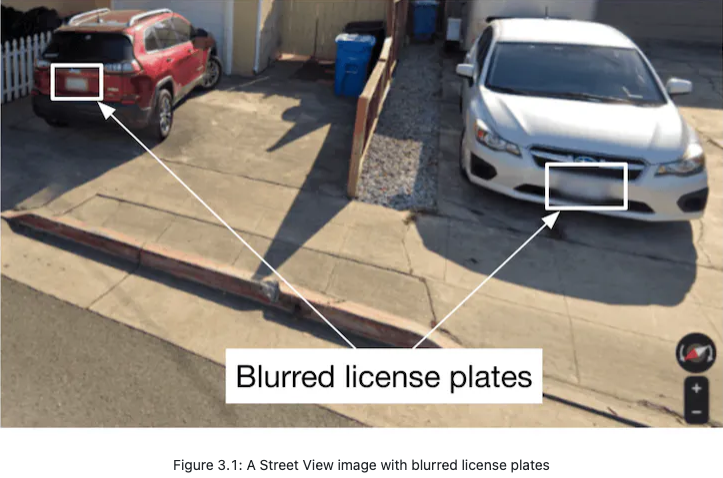
- Google Street View [1] is a technology in Google Maps that provides street-level interactive panoramas of many public road networks around the world. In 2008, Google created a system that automatically blurs human faces and license plates to protect user privacy. In this chapter, we design a blurring system similar to Google Street View.
Requirements
- Blur licence plates and human faces
- Let’s summarize the problem statement. We want to design a Street View blurring system that automatically blurs license plates and human faces. We are given a training dataset of 1 million images with annotated human faces and license plates. The business objective of the system is to protect user privacy.
ML Objective
- We want to detect objects of interest in an image.
- Blur the correctly detected objects
- The business objective of this system is to protect user privacy by blurring visible license plates and human faces in Street View images. But protecting user privacy is not an ML objective, so we need to translate it into an ML objective that an ML system can solve. One possible ML objective is to accurately detect objects of interest in an image. If an ML system can detect those objects accurately, then we can blur the objects before displaying the images to users.
- Throughout this chapter, we use “objects” instead of “human faces and license plates” for conciseness.
Specifying the system’s input and output
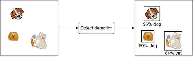
- The input of an object detection model is an image with zero or multiple objects at different locations within it. The model detects those objects and outputs their locations. Figure 3.2 shows an object detection system, along with its input and output.
Choosing the right ML category
- In general, an object detection system has two responsibilities:
- Predicting the location of each object in the image
- Predicting the class of each bounding box (e.g., dog, cat, etc.)
- The first task is a regression problem since the location can be represented by (x,y) coordinates, which are numeric values. The second task can be framed as a multi-class classification problem.
-
Traditionally, object detection architectures are divided into one-stage and two-stage networks. Recently, Transformer-based architectures such as DETR [2] have shown promising results, but in this chapter, we mainly explore two-stage and one-stage architectures.
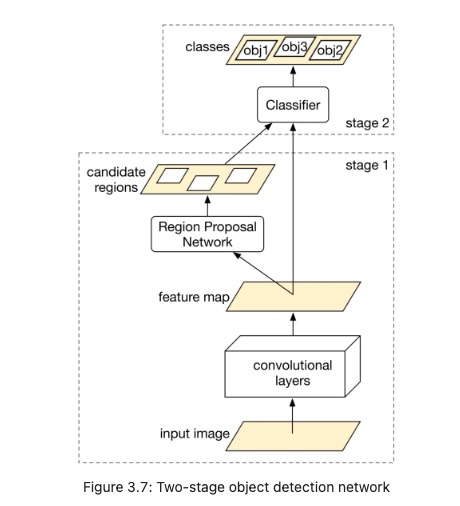
- Two-stage networks
-
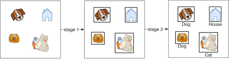
As the name implies, two separate models are used in two-stage networks:
- Region proposal network (RPN): scans an image and proposes candidate regions that are likely to be objects.
- Classifier: processes each proposed region and classifies it into an object class.
- One-stage networks
- In these networks, both stages are combined. Using a single network, bounding boxes and object classes are generated simultaneously, without explicit detection of region proposals. Figure 3.4 shows a one-stage network.
- Commonly used one-stage networks include: YOLO [6] and SSD [7] architectures.
- One-stage vs. two-stage
- Two-stage networks comprise two components that run sequentially, so they are usually slower, but more accurate.
- In our case, the dataset contains 1 million images, which is not huge by modern standards. This indicates that using a two-stage network doesn’t increase the training cost excessively. So, for this exercise, we start with a two-stage network. When training data increases or predictions need to be made faster, we can switch to one-stage networks.
System input and output
- Fed images
- Object detection
- output would be detected object and its location
High level overview
- Object detection I believe has two objectives:
- two options: R-CNN: two stage detection: performance
- First scans the image and proposes the location of each class
- Then runs a classifier on the proposed region and classifies it into the object class
- YOLO: one stage: latency
Data
- Do we have traffic images already, annotated
- Data engineering
- In the Introduction chapter, we discussed data engineering fundamentals. Additionally, it’s usually a good idea to discuss the specific data available for the task at hand. For this problem, we have the following data available:
- Annotated dataset
- Street View images
- Let’s discuss each in more detail.
- Annotated dataset
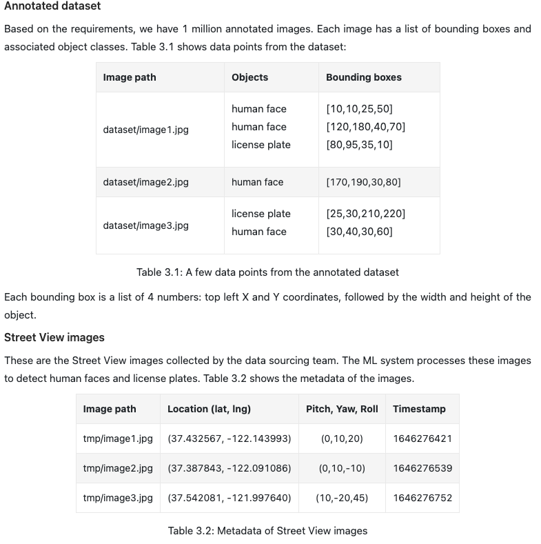
- Based on the requirements, we have 1 million annotated images. Each image has a list of bounding boxes and associated object classes.
- Each bounding box is a list of 4 numbers: top left X and Y coordinates, followed by the width and height of the object.
- Street View images
- These are the Street View images collected by the data sourcing team. The ML system processes these images to detect human faces and license plates. Table 3.2 shows the metadata of the images.
Feature engineering
-
During feature engineering, we first apply standard , such as resizing and normalization. After that, we increase the size of the dataset by using a data augmentation technique. Let’s take a closer look at this.
- Data augmentation
- A technique called data augmentation involves adding slightly modified copies of original data, or creating new data artificially from the original. As the dataset size increases, the model is able to learn more complex patterns. This technique is especially useful when the dataset is imbalanced, as it increases the number of data points in minority classes.
- A special type of data augmentation is image augmentation. Among the commonly used augmentation techniques are:
- Random crop
- Random saturation
- Vertical or horizontal flip
- Rotation and/or translation
- Affine transformations
- Changing brightness, saturation, or contrast
- It is important to note that with certain types of augmentations, the ground truth bounding boxes also need to be transformed. For example, when rotating or flipping the original image, the ground truth bounding boxes must also be transformed.
- Data augmentation is used in offline or online forms.
- Offline: Augment images before training
- Online: Augment images on the fly during training
- Online vs. offline: In offline data augmentation, training is faster since no additional augmentation is needed. However, it requires additional storage to store all the augmented images. While online data augmentation slows down training, it does not consume additional storage.
- The choice between online and offline data augmentation depends upon the storage and computing power constraints. What is more important in an interview is that you talk about different options and discuss trade-offs. In our case, we perform offline data augmentation.
- With preprocessing, images are resized, scaled, and normalized. With image augmentation, the number of images is increased. Let’s say the number increases from 1 million to 10 million.
Model Development
- Let’s examine each component.
- Convolutional layers
- Convolutional layers [9] process the input image and output a feature map.
- Region Proposal Network (RPN)
- RPN proposes candidate regions that may contain objects. It uses neural networks as its architecture and takes the feature map produced by convolutional layers as input and outputs candidate regions in the image.
- Classifier
- The classifier determines the object class of each candidate region. It takes the feature map and the proposed candidate regions as input, and assigns an object class to each region. This classifier is usually based on neural networks.
- In ML system design interviews, you are generally not expected to discuss the architecture of these neural networks.
Model Training
- Loss: Regression how aligned the predicted bounding boxes are with ground truth: MSE
- Classification, how accurate are the probabilities of the predicted objects vs the ground truth
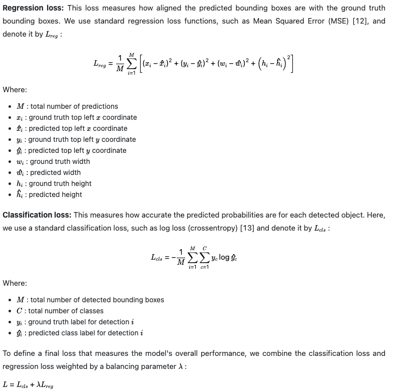
- The process of training a neural network usually involves three steps: forward propagation, loss calculation, and backward propagation. Readers are expected to be familiar with these steps, but for more information, see [11]. In this section, we discuss the loss functions commonly used to detect objects.
- An object detection model is expected to perform two tasks well. First, the bounding boxes of the objects predicted should have a high overlap with the ground truth bounding boxes. This is a regression task. Second, the predicted probabilities for each object class should be accurate. This is a classification task. Let’s define a loss function for each.
Evaluation
- Precision: Fraction of correct detections / all total detections its done
- During an interview, it is crucial to discuss how to evaluate an ML system. The interviewer usually wants to know which metrics you’d choose and why. This section describes how object detection systems are usually evaluated, and then selects important metrics for offline and online evaluations.
- An object detection model usually needs to detect N different objects in an image. To measure the overall performance of the model, we evaluate each object separately and then average the results.
- Figure 3.8 shows the output of an object detection model. It shows both the ground truth and detected bounding boxes. As shown, the model detected 6 bounding boxes, while we only have two instances of the object.

- When is a predicted bounding box considered correct? To answer this question, we need to understand the definition of Intersection Over Union.
- Intersection Over Union (IOU): IOU measures the overlap between two bounding boxes.
- IOU determines whether a detected bounding box is correct. An IOU of 1 is ideal, indicating the detected bounding box and the ground truth bounding box are fully aligned. In practice, it’s rare to see an IOU of 1 . A higher IOU means the predicted bounding box is more accurate. An IOU threshold is usually used to determine whether a detected bounding box is correct (true positive) or incorrect (false positive). For example, an IOU threshold of 0.7 means any detection that has an overlap of 0.7 or higher with a ground truth bounding box, is a correct detection.
- Now we know what IOU is and how to determine correct and incorrect bounding box predictions, let’s discuss metrics for offline evaluation.
Certainly, here’s a reformatted version:
Offline Metrics
Model development follows an iterative process, and offline metrics play a pivotal role in promptly gauging the performance of newly engineered models. For an object detection system, some significant metrics are:
- Precision
- Average Precision (AP)
- Mean Average Precision (mAP)
Precision
Precision signifies the ratio of accurate detections to all detections throughout all images. A high precision indicates the system’s reliability in its detections.
\[\text{Precision} = \frac{\text{Correct detections}}{\text{Total detections}}\]To compute precision, it’s essential to select an IOU threshold. Let’s elucidate with an example.
Figure 3.10 illustrates ground truth bounding boxes juxtaposed with detected bounding boxes and their respective IOUs.
Figure 3.10: Ground truth bounding boxes vs. detected bounding boxes
Evaluating precision for three varied IOU thresholds—0.7, 0.5, and 0.1—gives us:
-
IOU = 0.7: \(\text{Precision}_{0.7} = \frac{2}{6} = 0.33\)
-
IOU = 0.5: \(\text{Precision}_{0.5} = \frac{3}{6} = 0.5\)
-
IOU = 0.1: \(\text{Precision}_{0.1} = \frac{4}{6} = 0.67\)
A salient observation is that the precision fluctuates with different IOU thresholds, which makes discerning the model’s all-encompassing performance challenging using a singular precision score. AP offers a solution to this challenge.
Average Precision (AP)
- AP measures precision over an assortment of IOU thresholds and takes their average.
-
Here, \(P(r)\) denotes the precision at a particular IOU threshold, \(r\).
-
The integral can be estimated using a discrete summation over a fixed set of thresholds. For instance, the Pascal VOC2008 benchmark computes AP over 11 uniformly spaced threshold values.
Mean Average Precision (mAP)
- mAP signifies the average of AP across all object classes and provides an overview of the model’s comprehensive performance.
Where \(C\) is the total number of object classes the model can detect.
mAP is widely adopted for evaluating object detection systems. For specifics on thresholds employed in benchmarking, references [15] and [16] can be consulted.
Online Metrics
- Privacy of individuals is paramount, as per the system’s requirements. An effective approach to quantify this is by tallying user complaints and reports. Employing human annotators to periodically check the fraction of wrongly blurred images is also viable. Further, it’s vital to gauge metrics for bias and fairness. Ideally, human faces, irrespective of race or age group, should be blurred uniformly. However, measuring such biases, as per the stipulated requirements, is not included.
In Conclusion: For evaluation, while offline metrics rely on mAP and AP (with mAP offering a holistic view and AP detailing precision for specific classes), the main metric for online evaluation is user feedback through “user reports”.
Serving
- In this section, we first talk about a common problem that may occur in object detection systems: overlapping bounding boxes. Next, we propose an overall ML system design.
- Overlapping bounding boxes
- When running an object detection algorithm on an image, it is very common to see bounding boxes overlap. This is because the RPN network proposes various highly overlapping bounding boxes around each object. It is important to narrow down these bounding boxes to a single bounding box per object during inference.
- A widely used solution is an algorithm called “Non-maximum suppression” (NMS) [17]. Let’s examine how it works.
- A widely used solution is an algorithm called “” (NMS) [@nms]. Let’s examine how it works.
- NMS
- NMS is a post-processing algorithm designed to select the most appropriate bounding boxes. It keeps highly confident bounding boxes and removes overlapping bounding boxes.
- NMS is a commonly asked algorithm in ML system design interviews, so you’re encouraged to have a good understanding of it [18].
ML system design
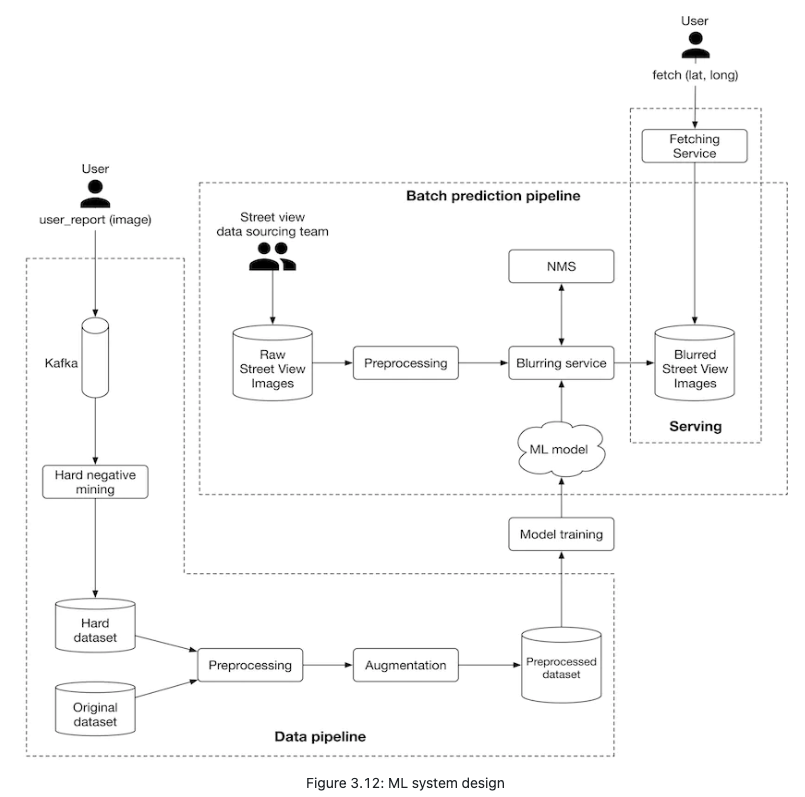
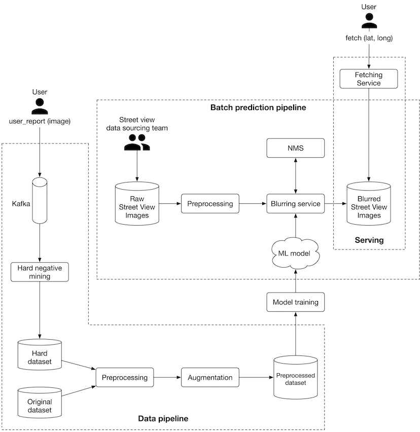
As illustrated in Figure 3.12, we propose an ML system design for the blurring system.
-
Let’s examine each pipeline in more detail.
- Batch prediction pipeline
- Based on the requirements gathered, latency is not a big concern because we can display existing images to users while new ones are being processed. Since instant results are not required, we can utilize batch prediction and precompute the object detection results.
- Preprocessing Raw images are preprocessed by this component. This section does not discuss the preprocess operations as we have already discussed them in the feature engineering section.
- Blurring service This performs the following operations on a Street View image:
- Provides a list of objects detected in the image.
- Refines the list of detected objects using the NMS component.
- Blurs detected objects.
- Stores the blurred image in object storage (Blurred Street View images).
- Note that the preprocessing and blurring services are separate in the design. The reason is preprocessing images tends to be a CPU-bound process, whereas blurring service relies on GPU. Separating these services has two benefits:
- Scale the services independently based on the workload each receives.
- Better utilization of CPU and GPU resources.
- Data pipeline
- This pipeline is responsible for processing users’ reports, generating new training data, and preparing training data to be used by the model. Data pipeline components are mostly self-explanatory. Hard negative mining is the only component that needs more explanation.
-
Hard negative mining. Hard negatives are examples that are explicitly created as negatives out of incorrectly predicted examples, and then added to the training dataset. When we retrain the model on the updated training dataset, it should perform better.
- Other Talking Points
- If time allows, here are some additional points to discuss:
- How Transformer-based object detection architectures differ from one-stage or twostage models, and what are their pros and cons [19].
- Distributed training techniques to improve object detection on a larger dataset [20] [21].
- How General Data Protection Regulation (GDPR) in Europe may affect our system [22].
- Evaluate bias in face detection systems [23] [24].
- How to continuously fine-tune the model [25].
- How to use active learning [26] or human-in-the-loop ML [27] to select data points for training.