Visual Search
- Overview
- Input/output
- High-level
- ML problem
- Choosing the right ML Category
- Data Preparation
- Feature engineering
- Model selection
- Model Training: Learning Image Representations
- Model Training Using SimCLR:
- Training Data Composition and Ground Truth
- Evaluation
- Testing
- Serving
- Prediction pipeline
- Re-ranking service
Overview
- A system helps users discover images that are visually similar to a selected image. In this chapter, we design a visual search system similar to Pinterest’s

Requirements
- Design a visual search system to retrieve simmilar images to the query image provided by the user.
- Rank on similartiy to the query image. Input is only images.
- In a conversation between a candidate and an interviewer about designing a visual search system:
- The system should rank results from most to least similar.
- The focus is only on images, not videos.
- The platform should allow users to select an image crop to retrieve similar images.
- There’s no need for personalization; all users see the same results for a given query image.
- While the model could use image metadata in practice, for this design, it will rely solely on image pixels.
- The only user action supported is image clicks, with features like save, share, or like excluded for simplicity.
- Content moderation isn’t a priority in this context.
- Training data can be constructed online based on user interactions.
- With an estimated 100-200 billion images on the platform, the search should be quick.
- In essence, the goal is to design a fast visual search system that displays images similar to a user’s query image, ranked by similarity. The system only caters to images and doesn’t involve personalization.
Input/output
- Input: the searched image
- Our system
- Output: ranked similar images
High-level
- Take the input image
- Transform it into an embedding, and have it in an embedding space
- We will try to find the similarity, cosine, dot product, what have you, this is how they are ranked
ML problem
- Rank images based on relevance/similarity
- Retrieve images similar to your query
- Frame the Problem as an ML Task
- In this section, we choose a well-defined ML objective and frame the visual search problem as an ML task.
- Defining the ML objective
- In order to solve this problem using an ML model, we need to create a well-defined ML objective. A potential ML objective is to accurately retrieve images that are visually similar to the image the user is searching for.
- Specifying the system’s input and output
- The input of a visual search system is a query image provided by the user. The system outputs images that are visually similar to the query image, and the output images are ranked by similarities. Figure 2.2 shows the input and output of a visual search system.
Choosing the right ML Category
- The output of the model is a set of ranked images that are similar to the query image. As a result, visual search systems can be framed as a ranking problem. In general, the goal of ranking problems is to rank a collection of items, such as images, websites, products, etc., based on their relevance to a query, so that more relevant items appear higher in the search results. Many ML applications, such as recommendation systems, search engines, document retrieval, and online advertising, can be framed as ranking problems. In this chapter, we will use a widely-used approach called representation learning. Let’s examine this in more detail.
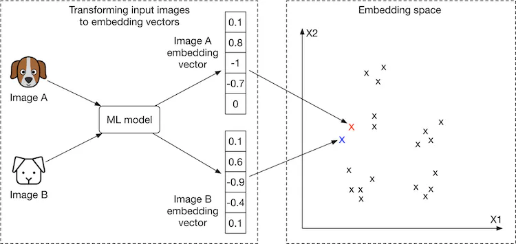
- Representation learning. In representation learning [3], a model is trained to transform input data, such as images, into representations called embeddings. Another way of describing this is that the model maps input images to points in an N-dimensional space called embedding space. These embeddings are learned so that similar images have embeddings that are in close proximity to each other, in the space. Figure 2.3 illustrates how two similar images are mapped onto two points in close proximity within the embedding space. To demonstrate, we visualize image embeddings (denoted by ‘x’) in a 2-dimensional space. In reality, this space is N-dimensional, where N is the size of the embedding vector.
- How to rank images using representation learning?
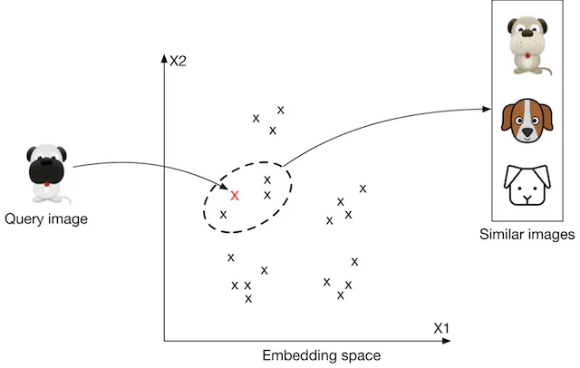
- First, the input images are transformed into embedding vectors. Next, we calculate the similarity scores between the query image and other images on the platform by measuring their distances in the embedding space. The images are ranked by similarity scores, as shown in Figure 2.4.
- At this point, you may have many questions, including how to ensure similar images are placed close to each other in the embedding space, how to define the similarity, and how to train such a model. We will talk more about these in the model development section.
Data Preparation
- Data engineering
- Aside from generic data engineering fundamentals, it’s important to understand what data is available. As a visual search system mainly focuses on users and images, we have the following data available:
- Images
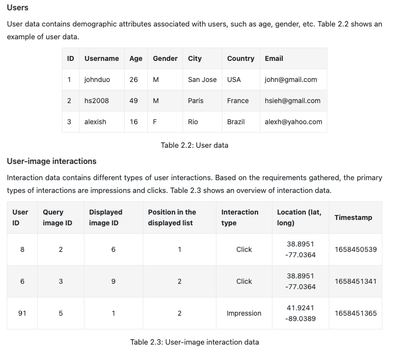
- Users
- User-image interactions
- Images
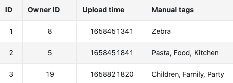
- Creators upload images, and the system stores the images and their metadata, such as owner id, contextual information (e.g., upload time), tags, etc. Table 2.1 shows a simplified example of image metadata.
Feature engineering
- In this section, we’ll delve into the process of engineering optimal features and preparing them for model ingestion. The nature of these features is predominantly influenced by our problem framing and the required model inputs.
-
Recall from the “Framing the problem as an ML task” segment, we approached the visual search system as a ranking challenge. We leveraged representation learning to address this, particularly utilizing a model that accepts an image as its input. However, prior to inputting into the model, the image necessitates some preprocessing. Here are some standard image preprocessing steps:
- Resizing: Models often demand fixed image dimensions, for instance, 224x224.
- Scaling: Adjust the image’s pixel values to fall within the 0 to 1 range.
- Z-score Normalization: Modify pixel values so they possess a mean of 0 and a variance of 1.
- Consistency in Color Mode: It’s crucial to maintain uniformity in the image’s color mode, be it RGB or CMYK.
Model selection
- Choosing Neural Networks
- The decision to opt for neural networks is based on the following reasons:
- Neural networks excel at processing unstructured data, which includes images and text.
- Contrary to several conventional machine learning algorithms, neural networks can generate the embeddings essential for representation learning. Suitable Neural Network Architectures
- The chosen architecture should be adept at handling image data. Architectures based on CNNs, like ResNet [4], or the newer Transformer-based structures, such as ViT [6], are known to be effective for image inputs.
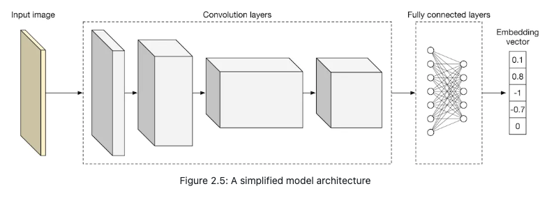
- Figure 2.5 depicts a basic model architecture that converts the input image into an embedding vector. Key hyperparameters to consider include the number of convolution layers, the neuron count in fully-connected layers, and the dimensions of the embedding vector. These are generally determined through experimental trials.
- CNN
- Input Image: This is where an image is fed into the network. The input image can be of various dimensions, but usually, it’s resized and normalized to a specific size before feeding into the model.
-
Convolution Layers: These are sequences of convolutional layers which process the input image. A convolution layer scans the input image with filters/kernels, capturing spatial information and producing feature maps. As we progress deeper through these layers, they capture more abstract features. In this diagram, the dimension of the feature map seems to reduce, indicating possible use of pooling layers or strided convolutions to reduce spatial dimensions while increasing depth (number of channels or feature maps).
-
Fully Connected Layers: After convolution layers, the output feature maps are often flattened or reshaped into a one-dimensional vector and then passed through one or more dense (fully connected) layers. These layers perform non-linear transformations of the extracted features and help in making final decisions or predictions.
-
Embedding Vector: The final output in this architecture is an embedding vector, which is a compact representation of the input image. The numbers shown (e.g., 0.1, 0.8, -1, -0.7, 0) are just illustrative values to represent the components of this vector. Embeddings are useful for tasks like image similarity, clustering, or any task where you want to have a dense, fixed-size representation of your input.
Model Training: Learning Image Representations
- For the retrieval of visually akin images, it’s crucial that our model learns representations, often termed as “embeddings”, during its training phase.
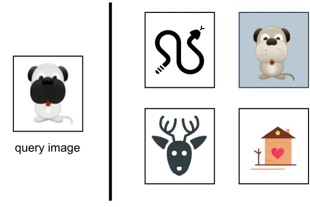
- A prevalent method employed for this learning is contrastive training [7]. Through this method, the objective is to train the model such that it can differentiate between similar and dissimilar images. As depicted in Figure 2.6:
- We supply the model with a query image (seen on the left).
- Alongside, we provide a similar image (as evidenced by the highlighted dog image on the right) and several dissimilar images.
- The essence of the training is to enable the model to create representations where the similar image aligns more closely to the query image in comparison to the other images showcased on the right in Figure 2.6.
Model Training Using SimCLR:
- SimCLR is a method that trains models using a contrastive learning approach.
- The main idea: Teach the model to recognize which images are similar and which are not.
- How it works:
- Take an image and create different versions of it using augmentations (like rotation).
- Train the model to recognize these augmented versions as similar to the original and different from other unrelated images.
- SimCLR stands for Simple Contrastive Learning of Visual Representations. It is a self-supervised learning framework developed by Google Research.
- The key idea is to train a neural network model to learn visual representations by contrasting positive and negative sample pairs.
- Positive pairs are created by applying data augmentations (like cropping, color distortion etc.) to the same image. Negative pairs are created using different images.
- In essence, SimCLR leverages image augmentations to help the model understand the core features of images and distinguish between similar and dissimilar images.
Training Data Composition and Ground Truth
Earlier, it was explained that each data point for training comprises:
- A query image.
- A positive image, which resembles the query.
- And, \(( n-1 )\) negative images that diverge from the query image.
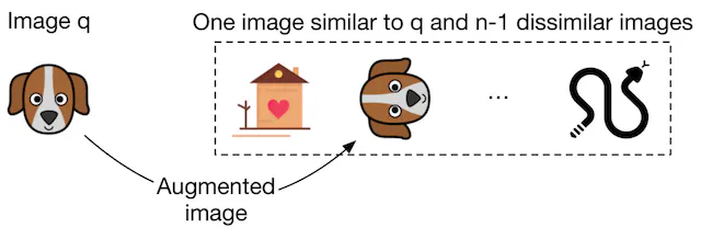
The ground truth label for a data point is essentially the index of its positive image. To illustrate, as shown in Figure 2.7:
- We present the model with a query image, denoted as ‘q’.
- Accompanying it, we have \(n\) images where one notably aligns with ‘q’ (as seen in the dog image).
-
The remaining \(n-1\) images stand as the negatives.
- For the given data point, the ground truth label is the index of the positive image, which in this case is \(2\) – denoting its position as the second among the \(n\) images in Figure 2.7.
- When creating a training data point, we typically pick a random query image alongside \(n-1\) images as negatives. For the selection of a positive image, we have three primary methods:
- Human Judgment
- Description: Engage human contractors to manually identify similar images.
- Pros: Delivers high accuracy in training data.
- Cons: It’s both costly and time-intensive.
- Using Interactions (like user clicks) as Indicators of Similarity
- Description: We infer similarity based on user interaction data. If a user clicks on an image, for instance, that clicked image is taken as analogous to the query image ‘q’.
- Pros: Automatic generation of training data; no manual intervention.
- Cons: Click data is inherently noisy. Users might click on unrelated images, and the dataset can be sparse. Using such inconsistent data might degrade the model’s performance.
- Artificially Generating a Similar Image from the Query Image (Self-Supervision)
- Description: From the query image, we artificially generate an analogous image (like through augmentation, e.g., rotation). Frameworks like SimCLR [7] and MoCo [8] adopt this methodology.
- Pros: Eliminates manual work and guarantees a related image since augmentation ensures similarity.
- Cons: The artificially constructed dataset can be distinct from real-life data. In reality, similar images aren’t just augmented versions of the query but are visually and contextually akin yet separate.
-
So, Which Method is Optimal?
- In an evaluative environment like interviews, it’s essential to outline multiple strategies and weigh their pros and cons. No one-size-fits-all solution exists. For our scenario, self-supervision stands out for two reasons:
- Absence of direct costs, thanks to its automation.
-
The success of frameworks like SimCLR [7] on vast datasets. Given our platform’s extensive image repository, this method seems apt.
- Nevertheless, should experimental results fall short, we have the flexibility to shift to other labeling methods. Starting with self-supervision and later incorporating click data for labeling could be a way. Merging methodologies is also viable. We could employ clicks for primary data formation and human annotators to weed out outliers or inconsistencies. Dialogue on these varied strategies and their implications with the interviewer is fundamental to make informed design choices.
- With the dataset prepared, we can proceed to model training using a suitable loss function.
Loss function
- Contrastive loss here:
- The loss function aims to minimize the distance between positive pairs in the embedding space while maximizing the distance between negative pairs.
- Some examples are NCE (Noise Contrastive Estimation) loss, triplet loss, InfoNCE loss etc. that are commonly used for contrastive representation learning.
-
Cross entropy to see how close the predicted probabilities are to the ground truth.
- Computing Similarities
- Initially, we must determine the similarities between the query image and embeddings of other images. The popular methods include:
- Dot Product [10]: A mathematical operation to measure similarity.
- Cosine Similarity [11]: Measures the cosine of the angle between two non-zero vectors.
-
Euclidean Distance [12]: Represents the linear distance between two points. However, in high dimensions, its efficacy dwindles due to the ‘curse of dimensionality’ [13]. For an in-depth understanding of this concept, refer to [14].
- Softmax Operation
-
Post computation of these distances, a softmax function is introduced. This function ensures that the resultant values coalesce to a sum of one, making it feasible to interpret these values as probabilities.
- Cross-Entropy
-
The cross-entropy metric [15] is used to gauge the proximity of the predicted probabilities to the actual, ground truth labels. If the predicted probabilities closely align with the ground truth, it implies that the embeddings aptly differentiate the positive image from its negative counterparts.
- Additional Insights for Interviews
- In a discussion setting, one might consider exploring the option of employing a pre-trained model. For instance, capitalizing on a pre-trained contrastive model and subsequently fine-tuning it with our training data could be a strategic move. The advantage? These pre-trained models have already been subjected to extensive datasets, enabling them to develop robust image representations. Consequently, this method offers a more time-efficient alternative than building a model from the ground up.
Evaluation
- Offline:
- Mean reciprocal rank (MRR): The average of the reciprocal ranks of the first correct answer in a list of results.
- Recall@k: Fraction of relevant items retrieved in the top-k results.
- Precision@k: Fraction of top-k results that are relevant.
- Mean average precision (mAP): Average precision scores for each query, often used in ranking or information retrieval tasks.
- Normalized discounted cumulative gain (nDCG): Measures the quality of a ranking, considering the position of relevant items and penalizing them if they appear lower in the list.
- Online:
- CTR
- Engagement: liked
- After developing the model, it’s essential to discuss its evaluation. This section elucidates the significant metrics for both offline and online evaluations.
Offline metrics
- An evaluation dataset, tailored to our requirements, is available for offline evaluation. Typically, each data point in this dataset comprises a query image, a set of candidate images, and a similarity score for each candidate-query image pair. The similarity score, an integer ranging from 0 to 5, indicates the extent of similarity: 0 for no similarity and 5 for high visual and semantic similarity. For each data point in the evaluation dataset, the ranking produced by the model is juxtaposed against the ideal ranking determined by the ground truth scores.
- In discussing offline metrics, it’s worthwhile to mention that these metrics are widely used not just in search systems but also in information retrieval and recommendation systems.
- Mean reciprocal rank (MRR)
-
- Formula:
\(MRR = \frac{1}{m} \sum_{i=1}^{m} \frac{1}{rank_{i}}\)
- Where \(m\) is the total number of output lists and \(rank_{i}\) represents the rank of the first relevant item in the ith output list.
- Figure 2.13: An illustration of MRR calculation.
- However, a major shortcoming of this metric is that it only considers the rank of the first relevant item in the output list, ignoring subsequent relevant items.
- Where \(m\) is the total number of output lists and \(rank_{i}\) represents the rank of the first relevant item in the ith output list.
- Formula:
\(MRR = \frac{1}{m} \sum_{i=1}^{m} \frac{1}{rank_{i}}\)
-
- Recall@k
- Formula: \(recall@k = \frac{\text{number of relevant items among the top k items in the output list}}{\text{total relevant items}}\) - The metric can sometimes be misleading, especially in systems where the total number of relevant items is extensive, which skews the recall metric.
- Precision@k
- Formula: \(precision@k = \frac{\text{number of relevant items among the top k items in the output list}}{k}\)
- Figure 2.15: A comparison of Precision@5 across two models. - This metric evaluates the precision of the output lists but does not account for ranking quality.
- Mean average precision (mAP)
- Formula for Average Precision (AP): \(AP = \frac{\sum_{i=1}^{k} \text{Precision@i if ith item is relevant}}{\text{total relevant items}}\)
- Figure 2.16: Illustration of mAP calculations. - mAP offers an average of precision values, hence considering the overall ranking quality of the list. However, its design is more suited for binary relevances.
- Normalized discounted cumulative gain (nDCG)
- DCG Formula: \(DCG_p = \sum_{i=1}^{p} \frac{rel_{i}}{log_{2}(i+1)}\) - Where \(rel_{i}\) is the relevance score of the image at the ith position. - * nDCG Formula: \(nDCG_p = \frac{DCG_p}{IDCG_p}\) - Where \(IDCG_p\) is the DCG of the ideally ranked list. * Figure 2.17: A sample list produced by a search system.
- nDCG, which measures the ranking quality, is pertinent for our evaluation since our dataset incorporates similarity scores.
Online metrics
-
This segment delves into several widely-adopted online metrics gauging the efficacy of image discovery for users.
- Click-through rate (CTR)
- Formula: \(CTR = \frac{\text{Number of clicked images}}{\text{Total number of suggested images}}\)
- CTR is an intuitive metric, indicating the frequency at which users engage with the displayed items.
Testing
- A/B testing
Serving
- ANN : FAISS and ScANN
Prediction pipeline
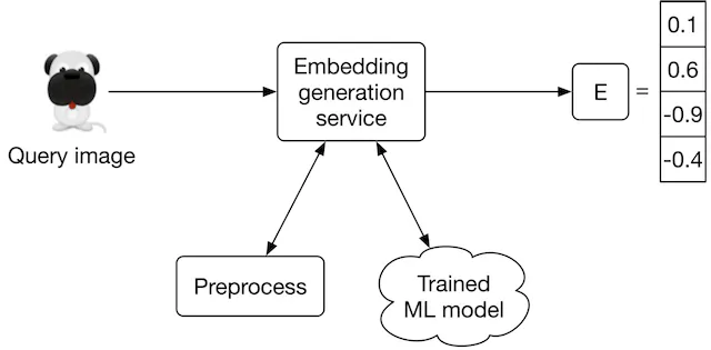
- Embedding generation service
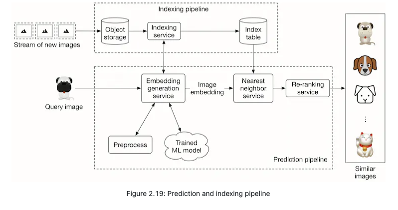
- This service computes the embedding of the input query image. As Figure 2.20 shows, it preprocesses the image and uses the trained model to determine the embedding.
Nearest neighbor service
- Once we get the embedding of the query image, we need to retrieve similar images from the embedding space. The nearest neighbor service does this.
- Let’s define the nearest neighbor search more formally. Given a query point “q” and a set of other points S, it finds the closest points to “q” in set S. Note that an image embedding is a point in N-dimensional space, where N is the size of the embedding vector. Figure 2.21 shows the top 3 nearest neighbors of image q. We denote the query image as q, and other images as x.
Re-ranking service
- This service incorporates business-level logic and policies. For example, it filters inappropriate results, ensures we don’t include private images, removes duplicates or nearduplicate results, and enforces other similar logic before displaying the final results to the user.
Indexing pipeline
Indexing service
- All images on the platform are indexed by this service to improve search performance.
- Another responsibility of the indexing service is to keep the index table updated. For example, when a creator adds a new image to the platform, the service indexes the embedding of the new image to make it discoverable by the nearest neighbor search.
- Indexing increases memory usage because we store the embeddings of the entire images in an index table. Various optimizations are available to reduce memory usages, such as vector quantization [16] and product quantization [17].
Performance of nearest neighbor (NN) algorithms
- Nearest neighbor search is a core component of information retrieval, search, and recommendation systems. A slight improvement in its efficiency leads to significant overall performance improvement. Given how critical this component is, the interviewer may want you to deep diver into this topic.
- NN algorithms can be divided into two categories: exact and approximate. Let’s examine each in more detail.
Exact nearest neighbor
- Exact nearest neighbor, also called linear search, is the simplest form of NN. It works by searching the entire index table, calculating the distance of each point with the query point q, and retrieving the k nearest points. The time complexity is O(N×D), where N is the total number of points and D is the point dimension.
- In a large-scale system in which N may easily run into the billions, the linear time complexity is too slow.
Approximate nearest neighbor (ANN)
- In many applications, showing users similar enough items is sufficient, and there is no need to perform an exact nearest neighbor search.
- In ANN algorithms, a particular data structure is used to reduce the time complexity of NN search to sublinear (e.g., O(D×logN). They usually require up-front preprocessing or additional space.
-
ANN algorithms can be divided into the following three categories:
- Tree-based ANN
- Locality-sensitive hashing (LSH)-based ANN
-
Clustering-based ANN
- There are various algorithms within each category, and interviewers typically do not expect you to know every detail. It’s adequate to have a high-level understanding of them. So, let’s briefly cover each category.
Tree-based ANN
- Tree-based algorithms form a tree by splitting the space into multiple partitions. Then, they leverage the characteristics of the tree to perform a faster search.
- We form the tree by iteratively adding new criteria to each node. For instance, one criterion for the root node can be: gender = male. This means any point with a female attribute belongs to the left sub-tree.
- In the tree, non-leaf nodes split the space into two partitions given the criterion. Leaf nodes indicate a particular region in space. Figure 2.23 shows an example of the space divided into 7 regions. The algorithm only searches the partition that the query point belongs to.
- Typical tree-based methods are R-trees [18], Kd-trees [19], and Annoy (Approximate Nearest Neighbor Oh Yeah) [20].
Locality sensitive hashing (LSH):
- LSH uses particular hash functions to reduce the dimensions of points and group them into buckets. These hash functions map points in close proximity to each other into the same bucket. LSH searches only those points belonging to the same bucket as the query point q. You can learn more about LSH by reading [21].
Clustering-based ANN
- These algorithms form clusters by grouping the points based on similarities. Once the clusters are formed, the algorithms search only the subset of points in the cluster to which the query point belongs.
Which algorithm should we use?
- Results from the exact nearest neighbor method are guaranteed to be accurate. This makes it a good option when we have limited data points, or if it’s required to have the exact nearest neighbors. However, when there are a large number of points, it’s impractical to run the algorithm efficiently. In this case, ANN methods are commonly used. While they may not return the exact points, they are more efficient in finding the nearest points.
- Given the amount of data available in today’s systems, the ANN method is a more pragmatic solution. In our visual search system, we use ANN to find similar image embeddings.
- For an applied ML role, the interviewer may ask you to implement ANN. Two widelyused libraries are Faiss [22] (developed by Meta) and ScaNN [23] (developed by Google). Each supports the majority of methods we have described in this chapter. You are encouraged to familiarize yourself with at least one of these libraries to better understand the concepts and to gain the confidence with which to implement the nearest neighbor search in an ML coding interview.
Other Talking Points
-
If there is extra time at the end of the interview, you might be asked follow-up questions or challenged to discuss advanced topics, depending on various factors such as the interviewer’s preference, the candidate’s expertise, role requirements, etc. Some topics to prepare for, especially for senior roles, are listed below.
- Moderate content in the system by identifying and blocking inappropriate images [24].
- Different biases present in the system, such as positional bias [25][26].
- How to use image metadata such as tags to improve search results. This is covered in Chapter 3 Google Street View Blurring System.
- Smart crop using object detection [27].
- How to use graph neural networks to learn better representations [28].
- Support the ability to search images by a textual query. We examine this in Chapter 4.
- How to use active learning [29] or human-in-the-loop [30] ML to annotate data more efficiently.
References
- Visual search at pinterest. https://arxiv.org/pdf/1505.07647.pdf.
- Visual embeddings for search at Pinterest. https://medium.com/pinterest-engineering/unifying-visual-embeddings-for-visual-search-at-pinterest-74ea7ea103f0.
- Representation learning. https://en.wikipedia.org/wiki/Feature_learning.
- ResNet paper. https://arxiv.org/pdf/1512.03385.pdf.
- Transformer paper. https://arxiv.org/pdf/1706.03762.pdf.
- Vision Transformer paper. https://arxiv.org/pdf/2010.11929.pdf.
- SimCLR paper. https://arxiv.org/pdf/2002.05709.pdf.
- MoCo paper. https://openaccess.thecvf.com/content_CVPR_2020/papers/He_Momentum_Contrast_for_Unsupervised_Visual_Representation_Learning_CVPR_2020_paper.pdf.
- Contrastive representation learning methods. https://lilianweng.github.io/posts/2019-11-10-self-supervised/.
- Dot product. https://en.wikipedia.org/wiki/Dot_product.
- Cosine similarity. https://en.wikipedia.org/wiki/Cosine_similarity.
- Euclidean distance. https://en.wikipedia.org/wiki/Euclidean_distance.
- Curse of dimensionality. https://en.wikipedia.org/wiki/Curse_of_dimensionality.
- Curse of dimensionality issues in ML. https://www.mygreatlearning.com/blog/understanding-curse-of-dimensionality/.
- Cross-entropy loss. https://en.wikipedia.org/wiki/Cross_entropy.
- Vector quantization. http://ws.binghamton.edu/fowler/fowler%20personal%20page/EE523_files/Ch_10_1%20VQ%20Description%20(PPT).pdf.
- Product quantization. https://towardsdatascience.com/product-quantization-for-similarity-search-2f1f67c5fddd.
- R-Trees. https://en.wikipedia.org/wiki/R-tree.
- KD-Tree. https://kanoki.org/2020/08/05/find-nearest-neighbor-using-kd-tree/.
- Annoy. https://towardsdatascience.com/comprehensive-guide-to-approximate-nearest-neighbors-algorithms-8b94f057d6b6.
- Locality-sensitive hashing. https://web.stanford.edu/class/cs246/slides/03-lsh.pdf.
- Faiss library. https://github.com/facebookresearch/faiss/wiki.
- ScaNN library. https://github.com/google-research/google-research/tree/master/scann.
- Content moderation with ML. https://appen.com/blog/content-moderation/.
- Bias in AI and recommendation systems. https://www.searchenginejournal.com/biases-search-recommender-systems/339319/#close.
- Positional bias. https://eugeneyan.com/writing/position-bias/.
- Smart crop. https://blog.twitter.com/engineering/en_us/topics/infrastructure/2018/Smart-Auto-Cropping-of-Images.
- Better search with gnns. https://arxiv.org/pdf/2010.01666.pdf.
- Active learning. https://en.wikipedia.org/wiki/Active_learning_(machine_learning).
- Human-in-the-loop ML. https://arxiv.org/pdf/2108.00941.pdf.