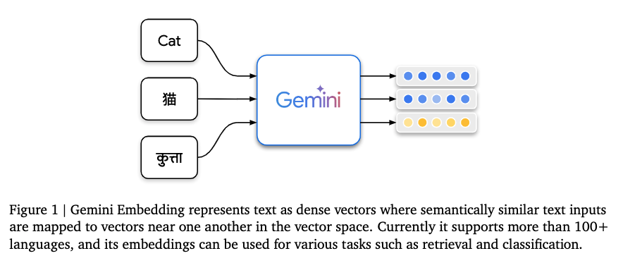
Gemini Embedding: Toward Universal Representations

Gemini Embedding: Toward Universal Representations

Background and scope

This primer summarizes the model design, training objective, data pipeline, and evaluation protocol of the Gemini Embedding model as described in the paper. It begins from the transformer-encoder view, presents the exact pooling/projection mechanics and loss, then covers the two-stage training recipe, data generation/filtering/mining, and evaluation setup.

Encoder architecture

Suppose the input sequence is

\[T = (t_1, t_2, \ldots, t_L),\]

a sequence of $L$ tokens after tokenization. Each token $t_i$ is mapped to an embedding vector and fed into a bidirectional transformer encoder $M$ (initialized from Gemini). The encoder outputs contextualized token embeddings:

\[T_{\text{embed}} = M(T) \in \mathbb{R}^{L \times d_M}.\]

Here, $d_M$ is the hidden size of the encoder. Each row $T_{\text{embed}}[i]$ corresponds to a token, but crucially, it is contextualized: the vector does not represent only the identity of $t_i$, but also how $t_i$ relates to every other token in the sequence.

This contextualization arises from the transformer’s self-attention mechanism, where each token embedding attends to the others and integrates information from them. As a result:

The vector for “bank” in “river bank” is pulled toward meanings related to water and geography.
The vector for “bank” in “savings bank” is shifted toward finance-related meanings. Both embeddings come from the same word, but they live in different parts of the hidden space because of their different contexts.

Mean pooling

The transformer outputs one vector per token, but for retrieval and similarity tasks, we need one sentence-level embedding. To do this, Gemini Embedding applies mean pooling across the token dimension:

\[P_{\text{embed}} = \frac{1}{L} \sum_{i=1}^{L} T_{\text{embed}}[i] \in \mathbb{R}^{d_M}.\]

Mean pooling computes the centroid of all token vectors, treating them as points in a high-dimensional space.

Intuitively, imagine every token embedding as a coordinate in $\mathbb{R}^{d_M}$. Mean pooling takes the geometric center of these points.
Theoretically, it is permutation-invariant: the result does not depend on token order (though token order already influenced the contextual vectors).
Statistically, it reduces variance and noise by averaging over all positions.

Example: In “The cat sat on the mat,” the words “cat,” “sat,” and “mat” each contribute their contextual embeddings. Averaging ensures the final representation reflects the sentence as a whole, rather than any single dominant word.

Alternatives to mean pooling

The paper chooses mean pooling deliberately. Other options include:

[CLS] pooling: use the representation of a special [CLS] token. This works in models like BERT, but performance often depends heavily on how the [CLS] token is trained. It may encode classification-specific signals rather than pure semantics.
Max pooling: take the maximum along each embedding dimension across tokens. This highlights the most salient features but can discard complementary information.
Attention pooling: learn a weighted average where some tokens contribute more. This can be powerful, but it introduces additional complexity and often requires supervision.

Mean pooling, in contrast, is simple, robust, and empirically stable across languages, tasks, and domains. It avoids overfitting to task-specific markers and produces embeddings that generalize well.

Linear projection

The pooled embedding is then passed through a linear projection:

\[E = f(P_{\text{embed}}) = W P_{\text{embed}} + b \quad \in \mathbb{R}^d,\]

where $W \in \mathbb{R}^{d \times d_M}$ and $b \in \mathbb{R}^d$.

This projection accomplishes two important functions:

Dimensional control: it allows the model to output embeddings of a chosen dimension $d$ (e.g., 768, 1536, 3072) without changing the encoder architecture.
Task alignment: it decouples the encoder’s hidden space (optimized for representation learning) from the final embedding space (optimized for similarity tasks).

Pipeline overview

Transformer encoder: contextualizes each token, producing vectors that encode both token identity and its relationships with the entire sequence.
Mean pooling: aggregates all contextualized vectors into one sentence-level representation by averaging.
Linear projection: reshapes this representation into the target embedding dimension, ensuring flexibility and task alignment.

The final vector (E) is the output embedding used for retrieval, clustering, or classification.

Training objective (contrastive NCE with in-batch negatives)

The Gemini embedding model is trained with a contrastive noise-contrastive estimation (NCE) loss. The goal is to pull queries and their correct targets closer together in the embedding space, while pushing them away from incorrect or irrelevant candidates.

Training example structure

Each training instance consists of:

A task string $t$, which tells the model what kind of problem it is solving (e.g., “question answering,” “retrieval,” “classification”).
A query $q_i$, such as a natural language question or a code snippet.
A positive target $p_i^{+}$, the correct answer passage or label.
Optionally, a hard negative $p_i^{-}$, which looks superficially similar to the positive but is actually incorrect.

Embedding step

The encoder maps both queries and targets into vectors using the same architecture described before (transformer → mean pooling → projection). For query $q_i$:

\[q_i = \text{mean\_pool}\left(M(t \oplus q_i)\right)\]

and for positives/negatives:

\[p_i^{\pm} = \text{mean\_pool}\left(M(p_i^{\pm})\right)\]

Here $t \oplus q_i$ denotes the concatenation of the task string and the query.

Similarity function

To compare vectors, the model uses cosine similarity:

\[\text{sim}(x,y) = \frac{x^\top y}{\lVert x \rVert \lVert y \rVert}\]

Cosine similarity measures the angle between two vectors, ignoring their length. This is particularly useful for embeddings, where direction in space matters more than raw magnitude.

Loss function

For a batch of size $B$, the training uses in-batch negatives: every other pair in the same batch serves as a negative example for the current query. This greatly increases training efficiency, since one batch provides $B^2$ comparisons instead of just $B$.

With temperature $\tau$, the per-example loss is:

\[\mathcal{L}_i = -\log \frac{\exp\left(\frac{\text{sim}(q_i, p_i^{+})}{\tau}\right)} {\mathbf{1}_{\{\text{hard neg present}\}}\exp\left(\frac{\text{sim}(q_i, p_i^{-})}{\tau}\right) + \sum_{j=1}^{B} \text{mask}(i,j)\exp\left(\frac{\text{sim}(q_i, p_j^{+})}{\tau}\right)}.\]

The total batch loss is:

\[\mathcal{L} = \frac{1}{B} \sum_{i=1}^{B} \mathcal{L}_i\]

Intuition

Numerator: the similarity between the query and its correct positive. The loss is minimized when this similarity is high.
Denominator: the sum of similarities with negatives (all other positives in the batch, plus any explicit hard negative). The loss is minimized when these similarities are low.
Temperature $\tau$: controls how sharply the softmax weights similarities. A smaller $\tau$ makes the model focus more strongly on the hardest negatives.

Role of hard negatives

Hard negatives are particularly tricky examples (e.g., a passage that looks like the right answer but isn’t). By explicitly including them in the denominator, the model learns fine-grained distinctions.

However, the paper notes that adding too many hard negatives can hurt, the model starts overfitting to distinguishing subtle noise rather than learning broad semantic separation.

Example

Suppose we are training on the query:

“Who wrote the play Hamlet?”

Positive $p_i^{+}$: “William Shakespeare authored Hamlet, one of his most famous tragedies.”
Hard negative $p_i^{-}$: “Hamlet is one of the most frequently performed plays in the world.”

The hard negative is topically correct (it’s about Hamlet), but it doesn’t answer the question. Training pushes the query embedding closer to the positive and away from both the hard negative and other batch candidates (e.g., answers about Moby-Dick or The Odyssey).

Masking and “same-tower negatives”

The mask function ensures degenerate cases are excluded:

For classification, the same label appearing in the batch is not counted as a negative.
“Same-tower negatives” (examples encoded by the same side of the model) are omitted, since they often produce false negatives that degrade performance.

Multi-resolution training for multiple output dimensions (MRL)

A challenge in embedding models is that different applications have different requirements for embedding dimensionality.

High-dimensional embeddings (e.g., 3072-dim) capture more information and perform better on fine-grained semantic tasks, but they are computationally expensive to store, index, and compare.
Low-dimensional embeddings (e.g., 768-dim) are cheaper and faster, but may sacrifice accuracy.

Normally, one would train and maintain multiple models for different embedding sizes. Gemini Embedding avoids this duplication by using Matryoshka Representation Learning (MRL), where a single model can serve multiple embedding sizes at once.

How MRL works

The idea is to train the embedding space such that prefix slices of the full embedding vector are themselves valid embeddings.

Suppose the model outputs a full embedding $E \in \mathbb{R}^{3072}$.
With MRL, the first 768 dimensions $E_{1:768}$ should already be a strong embedding; likewise the first 1536 dimensions $E_{1:1536}$.
This is achieved by adding multiple contrastive losses during training, one per prefix.

Formally, if $\mathcal{L}^{d}$ denotes the contrastive loss computed on the first $d$ dimensions of the embedding, then the total loss is:

\[\mathcal{L}_{\text{MRL}} = \sum_{d \in \{768,1536,3072\}} \mathcal{L}^{d}\]

This forces the model to distribute semantic information across the vector in a layered way, like a nested set of dolls (hence “Matryoshka”).

Intuition

Efficiency: At inference time, the same trained model can output 768-, 1536-, or 3072-dim embeddings by truncating.
Flexibility: Users can trade accuracy for speed depending on their application, without retraining.
Representation sharing: Lower-dimensional embeddings act as compressed summaries, while higher dimensions capture finer distinctions.

Two-stage training recipe

Gemini Embedding training is not a single pass. Instead, it follows a two-stage curriculum: pre-finetuning followed by finetuning, with an additional ensemble-like averaging step called “model soup.”

1. Pre-finetuning

Purpose: Adapt the Gemini language model (trained for autoregressive generation) into an encoder suitable for embeddings.
Data: A very large, noisy collection of (query, target) pairs. These are not carefully curated but provide broad coverage.
Batch size: Very large. Larger batches help stabilize the contrastive loss, since each batch provides many in-batch negatives.
Negatives: Hard negatives are not used at this stage; the model relies on random in-batch negatives.
Duration: This stage is run for significantly longer than finetuning, allowing the model to acquire a general embedding capability.

Think of this as roughly sculpting the embedding space: not perfect, but shaped enough to separate broadly correct vs. incorrect matches.

2. Finetuning

Purpose: Refine the pre-finetuned encoder on carefully chosen datasets to maximize performance on downstream tasks.
Mixture composition: Designed to balance
- task diversity (e.g., retrieval, classification, clustering),
- language diversity (over 250 languages), and
- code retrieval (so embeddings work well on source code).
Batch size: Smaller than pre-finetuning. Each batch is drawn from a single dataset, which sharpens the contrastive signal by forcing the model to discriminate examples within that domain.
Hyperparameters: Learning rates, mixture weights, and other factors are tuned systematically (e.g., grid search).
Outputs: Multiple candidate checkpoints, each representing a different mixture/hyperparameter setting.

This stage is like polishing the embedding space: ensuring the model captures nuanced semantic differences across tasks and languages.

3. Model soup

After finetuning, the team doesn’t just pick one checkpoint. Instead, they apply a parameter averaging strategy known as “model soup”:

Multiple finetuned checkpoints (from different runs, hyperparameters, or datasets) are combined by averaging their weights.
Averaging can be uniform (simple mean) or weighted (emphasizing stronger runs).
The result is a model that often generalizes better than any individual checkpoint, smoothing out idiosyncrasies from specific runs.

This final step can be thought of as ensembling without extra cost: a single averaged model retains much of the diversity of multiple fine-tuned ones.

Data pipeline enhancements using Gemini

Synthetic data generation Additional retrieval and classification data are generated with few-shot prompting. For retrieval, the paper extends prior synthetic-query pipelines (e.g., FRet and SWIM-IR adaptations) to generate queries for web passages, followed by an automatic rating step to filter low-quality generations. For classification, synthetic datasets (e.g., counterfactual, sentiment, reviews) are produced. Multi-stage prompting (e.g., conditioning on synthetic user/product/movie metadata and sampling from longer candidate lists) is used to improve realism and diversity.
LLM-based data filtering Human-annotated retrieval datasets can contain incorrect positives/negatives. The paper uses Gemini to score and filter out low-quality examples via few-shot prompting for data quality assessment.
Hard negative mining A Gemini-initialized embedding model is first trained without hard negatives. For each query, a set of nearest-neighbor candidates is retrieved. Each candidate is then scored with two prompting strategies (graded classification and query likelihood), and the scores are fused using Reciprocal Rank Fusion (RRF). The lowest-scoring neighbor among these fused ranks is selected as the hard negative. The paper observes that adding some hard negatives improves retrieval metrics, but adding too many leads to overfitting.

Evaluation setup and findings (paper summary)

The model is evaluated across Massive Multilingual Text Embedding Benchmark (MMTEB), including multilingual, English, and code tracks; and on cross-lingual retrieval benchmarks XOR-Retrieve and XTREME-UP.
The paper reports state-of-the-art aggregate performance on MTEB(Multilingual) at the time of submission, and strong results on MTEB(Eng, v2), MTEB(Code), and cross-lingual retrieval.
The ablations show: pre-finetuning materially improves results; mixtures emphasizing task diversity are especially important; multilingual finetuning most helps long-tail languages; filtering MIRACL training data improves retrieval in many languages; and hard-negative counts should be moderated to avoid overfitting.

Practical shape of the model interface (as described)

Inputs Text sequences with an optional task string prefix (t) can be encoded.
Encoder Bidirectional transformer (M) (initialized from Gemini).
Pooling Mean pooling over tokens.
Projection Linear map $f:\mathbb{R}^{d_M} \to \mathbb{R}^{d}$ with $d \in {768,1536,3072}$ supported via MRL.
Similarity Cosine similarity $\text{sim}(x,y)=\frac{x^\top y}{\lVert x\rVert \lVert y\rVert}$.
Loss Contrastive NCE with in-batch negatives, an optional explicit hard negative, masking for classification-style batches, and temperature $\tau$.
Training recipe Pre-finetuning → finetuning mixtures → model soup.

Full loss written end-to-end (with temperature and masking)

Let:

$S_i^+ = \exp(\text{sim}(q_i,p_i^{+})/\tau)$
$S_i^- = \mathbf{1}_{{\text{hard neg present}}}\exp(\text{sim}(q_i,p_i^{-})/\tau)$
$S_{ij} = \text{mask}(i,j)\exp(\text{sim}(q_i,p_j^{+})/\tau)$

Then

\[\mathcal{L} = \frac{1}{B}\sum_{i=1}^{B} \left[ -\log \frac{S_i^+}{S_i^- + \sum_{j=1}^{B} S_{ij}} \right]\]

Where:

$\mathcal{L}$ is the total batch loss
$S_i^+$ is the similarity with the positive example
$S_i^-$ is the similarity with the hard negative (if present)
$S_{ij}$ is the similarity with other examples in the batch

With MRL, this loss is computed on several prefix slices of the embedding and summed.

Closing summary

The paper’s core design can be read succinctly as: Gemini-initialized bidirectional transformer encoder → mean pooling → linear projection; trained with a contrastive NCE loss using in-batch negatives plus carefully mined hard negatives; multi-resolution losses to support multiple output sizes in one model; two-stage training and model-soup averaging; and data quality improvements via synthetic generation, LLM filtering, and RRF-based hard-negative mining. The reported evaluations show strong multilingual, English, code, and cross-lingual retrieval performance under this recipe.