Primers • Continuous Autoregressive Language Models
- Motivation: The Limits of Token-by-Token Autoregression
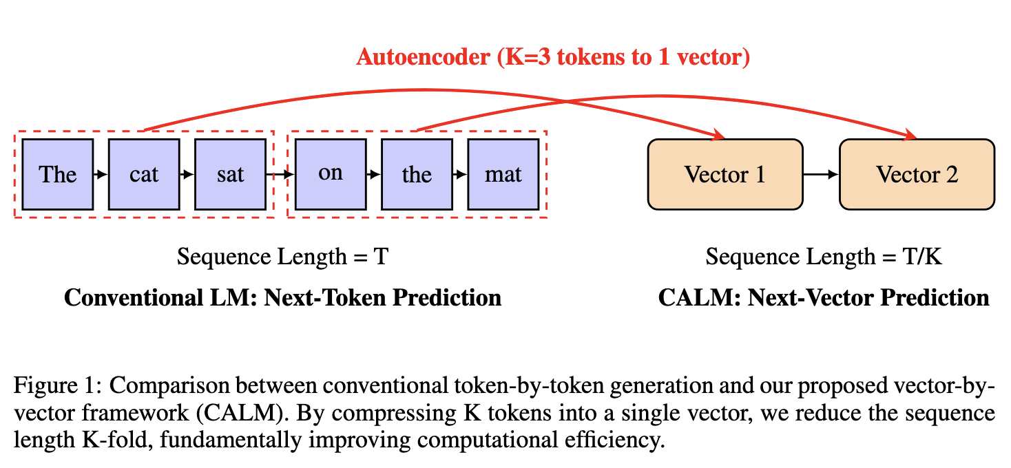
- From Tokens to Vectors: The CALM Paradigm
- The Architecture of Continuous Autoregression
- Modeling in Continuous Space
- Energy-Based Generative Modeling and Evaluation
- Training and Empirical Insights
- Broader Implications and Theoretical Connections
Motivation: The Limits of Token-by-Token Autoregression
Large language models rely on a discrete autoregressive factorization of the joint probability of a sequence:
\[p(x_{1:T}) = \prod_{t=1}^{T} p(x_t \mid x_{<t})\]Notation and variables for the factorization:
- $x_{1:T}$: a length–$T$ discrete sequence of tokens. Indexing is 1 based.
- $x_t \in {1,\dots,V}$: the token identity at time step $t$, expressed as a vocabulary index.
- $x_{<t} := (x_1,\dots,x_{t-1})$: the prefix of tokens strictly before position $t$.
- $V$: the vocabulary size, that is, the number of unique token types the model can emit.
- $p(\cdot)$: a probability mass function over token identities.
- The product expands the chain rule of probability: each conditional $p(x_t \mid x_{<t})$ is a categorical distribution that depends on the entire prefix.
Each term is parameterized by a neural network that computes a contextual hidden representation and then projects to the probability simplex:
\[p(x_t \mid x_{<t}) = \text{softmax}(W h_t)\]Definitions for the softmax parameterization:
- $h_t = f_\theta(x_{<t}) \in \mathbb{R}^{d}$: the hidden state produced by a transformer with parameters $\theta$ given the prefix $x_{<t}$. The mapping $f_\theta$ includes token embeddings, positional encodings, attention and feedforward layers, and layer normalizations.
- $d$: the hidden width of the transformer, that is, the dimensionality of $h_t$.
- $W \in \mathbb{R}^{V \times d}$: the output projection matrix that maps $h_t$ to unnormalized logits $o_t = W h_t \in \mathbb{R}^{V}$.
- $\text{softmax}(o)i = \exp(o_i) \big/ \sum{j=1}^{V} \exp(o_j)$: converts logits to a categorical probability distribution over the $V$ token identities.
- $p(x_t \mid x_{<t}) \in \Delta^{V-1}$: a point on the $(V-1)$ dimensional probability simplex.
This architecture is exact and tractable, but it is also restrictive: generation proceeds strictly left to right and communicates information using single discrete symbols.
This primer is based on the recent paper, “Continuous Autoregressive Language Models” by Tencent and Tsinghua
The Sequential Bottleneck
Autoregressive decoding imposes a linear-time dependency on sequence length because each token requires conditioning on all prior tokens. Even with key value caching that reuses attention keys and values from earlier steps, decoding remains serial: the model emits exactly one token per forward step.
Two bottlenecks arise:
-
Computation: generation cost scales as $O(T)$ for a sequence of length $T$. Each emitted token triggers at least one pass through the top layers of the network plus the output projection. With caching, attention cost per new token is $O(L d)$ for $L$ layers and width $d$, but the number of steps still grows linearly with $T$.
-
Information: each step emits one categorical symbol with at most $\log_2 V$ bits of instantaneous capacity, regardless of the internal representational richness of $h_t$.
As models scale in depth and width, $h_t$ becomes a high capacity carrier of semantics, but the output channel remains a single discrete decision per step. This mismatch grows with model scale and context length.
Semantic Bandwidth and Information Density
Let the hidden state at time $t$ be a continuous random variable and the emitted token be discrete:
- $H_t \in \mathbb{R}^{d}$: the random variable induced by $h_t = f_\theta(X_{<t})$ when the input prefix is drawn from a data distribution.
- $X_t \in {1,\dots,V}$: the token identity random variable at time $t$.
- $X_{<t}$: the random token prefix.
Define the semantic bandwidth, the rate at which internal semantics are communicated to the output:
\[\mathcal{B}_t = I(H_t; X_t \mid X_{<t})\]Definitions for $\mathcal{B}_t$:
- $I(A;B \mid C)$: conditional mutual information, that is, the expected reduction in uncertainty about $B$ when observing $A$, given $C$.
- $\mathcal{B}t$ measures how many bits of information about the emitted token $X_t$ are actually carried by the hidden state $H_t$ beyond what is already known from the prefix $X{<t}$.
Because $X_t$ is categorical with at most $V$ outcomes:
\[\mathcal{B}_t \leq H(X_t \mid X_{<t}) \leq \log V\]Additional clarifications:
- $H(\cdot)$ denotes Shannon entropy in nats if the logarithm is natural or in bits if base 2. Here the inequality is stated in nats or bits consistently with the logarithm base.
- The upper bound $\log V$ is the maximal entropy of a categorical variable with $V$ outcomes.
- In natural language, $H(X_t \mid X_{<t})$ is typically much smaller than $\log V$ because the next token distribution is highly peaked under realistic contexts.
By contrast, the internal state $H_t$ is continuous and high dimensional. If values are represented at precision $\epsilon$ per dimension, the effective information capacity of $H_t$ scales on the order of $d \log_2(1/\epsilon)$ bits. Therefore a large information reservoir is compressed into a single discrete symbol at each step. This implies an information rate mismatch: the model’s internal channel capacity significantly exceeds the rate at which it can emit semantic content.
Why Expanding Vocabulary Size Fails
A naive remedy is to enlarge $V$ so that each token could, in principle, convey more information. This creates several systemic issues.
Computational cost:
- The softmax normalization $\sum_{j=1}^{V} \exp(o_{t,j})$ grows linearly with $V$. Even when using sampled softmax or adaptive softmax, the cost and complexity of training and inference increase with $V$.
Gradient noise and estimation stability:
Consider the gradient of the log likelihood for a single step:
\[\nabla_\theta \log p(x_t \mid x_{<t}) = \nabla_\theta h_t^\top \Big( W_{x_t} - \mathbb{E}_{y \sim p(\cdot \mid x_{<t})}[W_y] \Big)\]Variable definitions and implications:
- $W_{x_t} \in \mathbb{R}^{d}$: the row of $W$ corresponding to the true token $x_t$.
- $\mathbb{E}{y \sim p(\cdot \mid x{<t})}[W_y] = \sum_{y=1}^{V} p(y \mid x_{<t}) W_y$: the probability weighted average of all rows of $W$.
- As $V$ increases, the support of $p(\cdot \mid x_{<t})$ becomes wider, and even if the distribution is peaked, the normalization and the expectation involve many rows. The signal to noise of the difference $W_{x_t} - \mathbb{E}[W]$ degrades in practice due to numerical and sampling considerations.
- If one uses approximations such as sampled softmax, bias and variance of the estimator worsen with $V$ unless the number of samples also scales, which raises compute cost.
Statistical inefficiency:
- Natural language token frequencies are heavy tailed. Increasing $V$ introduces many rare types that are poorly estimated, hurting generalization and calibration.
- Larger $V$ increases embedding and output head parameters, raising memory footprint and the risk of overfitting on rare entries.
Empirically, perplexity improvements plateau beyond moderate vocabulary sizes, indicating that the limitation is structural: single token emission per step constrains the usable semantic throughput, regardless of $V$.
The Continuous Representation Hypothesis
The core inefficiency stems from discrete emission. A more expressive formulation operates in continuous space so that each step can encode multiple tokens worth of information in a single vector.
Let a latent vector carry the semantics of a local text segment:
- $z_t \in \mathbb{R}^{d_z}$: a continuous latent representing a chunk of future text around step $t$.
- $d_z$: the dimensionality of the latent space, which may differ from the transformer width $d$.
Define a continuous autoregressive process over the latent sequence:
\[p(z_{1:T}) = \prod_{t=1}^{T} p(z_t \mid z_{<t})\]Explanations:
- $z_{1:T}$ here denotes a sequence of $T$ latent vectors used for exposition. In practice one often has $M$ latent steps for $T$ tokens with a compression factor $K = T/M$.
- $p(z_t \mid z_{<t})$ is a conditional distribution over $\mathbb{R}^{d_z}$, not a categorical distribution. It can be parameterized without a softmax, for example by an energy based sampler or another likelihood free mechanism.
To surface tokens from latents, introduce a learned decoder $g_\phi$:
\[x_{1:K_t} = g_\phi(z_t)\]where:
- $g_\phi: \mathbb{R}^{d_z} \rightarrow {1,\dots,V}^{K_t}$ maps a single latent to a short token sequence.
- $K_t \in \mathbb{N}$: the number of tokens reconstructed from $z_t$. It may be fixed to $K$ or allowed to vary with local content.
- The decoder can be implemented by the decoder half of a text autoencoder trained for high fidelity reconstruction.
This establishes a continuous autoregressive language model: at each step the model predicts a semantic vector rather than a token identity. The categorical bottleneck is removed during prediction, and multiple tokens can be reconstructed from one latent.
Effective semantic bandwidth increases because each step carries an entire chunk’s worth of information. When $K$ tokens are reconstructed per latent, the number of autoregressive steps needed to produce a length–$T$ sequence reduces from $T$ to approximately $T/K$.
Speculative Decoding as an Intermediate Solution
Speculative decoding partially mitigates sequential dependence within the discrete paradigm by decoupling proposal and verification. A small draft model proposes candidate tokens in parallel and a larger target model verifies them.
Let
- $p_{\text{draft}}(\cdot \mid \cdot)$: the proposal distribution of the draft model.
- $p_{\text{target}}(\cdot \mid \cdot)$: the verification d_
From Tokens to Vectors: The CALM Paradigm
Continuous Autoregressive Language Models (CALMs) redefine the granularity of prediction. Instead of emitting one discrete token at a time, the model predicts a continuous latent vector that encapsulates the semantic content of several future tokens. This section describes the theoretical basis for that representation: how discrete sequences are mapped to latent vectors, how those vectors are trained to preserve meaning, and why this allows the model to predict at a higher semantic bandwidth.
The Autoencoding Foundation
The transition from discrete to continuous representation begins with a text autoencoder. An autoencoder learns an invertible mapping between discrete token sequences and continuous vectors that preserve linguistic information.
We consider a text sequence
\(x_{1:T} = (x_1, x_2, \dots, x_T),\)
where each $x_t$ is a discrete symbol from the vocabulary $\mathcal{V}$ of size $V$.
The autoencoder defines two transformations:
-
Encoder $E_\phi$: compresses text into a sequence of latent vectors
\(z_{1:M} = E_\phi(x_{1:T}),\)
where $M \ll T$. Each $z_i \in \mathbb{R}^{d_z}$ is a dense vector summarizing roughly $K = T/M$ tokens. -
Decoder $D_\psi$: reconstructs text from latents
\(\hat{x}_{1:T} = D_\psi(z_{1:M}).\)
The encoder compresses multiple discrete symbols into one latent representation, while the decoder expands these continuous representations back to tokens. Training jointly on reconstruction ensures that $z_i$ retains all information needed to reproduce the underlying text segment.
The autoencoder objective is the negative log-likelihood of reconstruction: \(\mathcal{L}_{\text{rec}}(\phi, \psi) = -\mathbb{E}_{x_{1:T} \sim \mathcal{D}} \left[\sum_{t=1}^{T} \log p_\psi(x_t \mid z_{1:M})\right],\) where $\mathcal{D}$ is the text corpus and $p_\psi$ is the decoder’s predictive distribution over tokens.
In practice, the decoder need not be probabilistic in the standard language modeling sense; it can be viewed as a deterministic or energy-based reconstruction network. What matters is that the learned latent space preserves enough local smoothness for gradients to propagate and for nearby vectors to represent semantically similar text.
Compression and Semantic Representation
Compression introduces a new axis of modeling capacity. In the discrete autoregressive regime, every token is its own atomic prediction. In CALM, the encoder determines how many tokens $K$ each latent should represent.
High compression (large $K$) forces the model to summarize several words, phrases, or syntactic patterns into one vector. The resulting latent space behaves like a semantic manifold, where distances encode meaning similarity rather than token-level proximity.
Each latent $z_i$ therefore captures a semantic chunk: a local region of meaning that spans several tokens but remains short enough to maintain syntactic coherence. In practice, this chunking can emerge organically through the autoencoder objective — the network learns the scale of compression that minimizes reconstruction loss while maintaining smoothness in latent space.
Structure of the Latent Space
The latent space must satisfy three theoretical properties to support autoregression:
- Continuity: small changes in latent vectors correspond to small changes in decoded text. This allows the generative model to operate smoothly and to interpolate between meanings.
- Disentanglement: different latent dimensions should capture distinct semantic factors such as content, syntax, and style. Perfect disentanglement is impossible, but approximate independence improves stability.
- Invertibility: decoding from latents back to text must be well-posed; the mapping $D_\psi$ should be approximately bijective over the data manifold.
A useful conceptual view is to treat the latent space as a semantic coordinate system of language. The encoder assigns each text segment a coordinate vector $z_i$ whose geometry encodes the structure of meaning. The decoder then acts as a differentiable interpreter that maps coordinates back to surface forms.
Regularization and Stability
Without additional constraints, an autoencoder can collapse: the encoder might map many different text segments to the same region of latent space, or the decoder might memorize the training data rather than learning a structured inverse. CALM-style autoencoders employ regularization to avoid these degeneracies.
-
Variational constraints:
Introduce a prior distribution $p(z)$, often standard normal, and penalize deviation of the posterior $q_\phi(z \mid x)$ from the prior using the KL divergence. This keeps the latent distribution compact and isotropic, improving smoothness and preventing unbounded drift. -
Noise robustness:
Add stochastic perturbations during encoding, $z = E_\phi(x) + \epsilon$, with $\epsilon \sim \mathcal{N}(0, \sigma^2 I)$. This trains the decoder to tolerate slight errors in latent prediction — crucial for the downstream autoregressive model, which must predict these latents continuously. -
Information balance:
Weight the KL penalty or noise level to balance reconstruction fidelity and generalization. If the latent dimension is large or the regularization too weak, the autoencoder can overfit and produce non-smooth latents that the autoregressive model cannot model effectively.
The outcome is a latent space that is continuous, regularized, and reconstructable — the necessary substrate for continuous autoregressive modeling.
Encoding Multiple Tokens per Step
Once trained, the encoder provides a deterministic compression mapping from text to latents: \(z_i = f_{\text{enc}}(x_{iK - K + 1 : iK}),\) where $K$ denotes the number of tokens represented by one latent vector. The decoder performs the approximate inverse mapping: \(\hat{x}_{iK - K + 1 : iK} = f_{\text{dec}}(z_i).\)
This establishes a semantic quantization of text: instead of discrete tokens, language is represented as a sequence of dense vectors, each summarizing a coherent linguistic unit. Unlike Byte Pair Encoding or WordPiece tokenization, this quantization is learned directly from data and optimized for reconstruction and generative modeling.
Importantly, these continuous chunks preserve dependencies beyond token boundaries. Because the encoder can use contextual attention across chunk boundaries, $z_i$ depends not only on its local tokens but also on preceding and following context. This yields context-aware latents that better reflect the semantics of natural language.
From Autoencoding to Autoregression
With a stable autoencoder in place, CALM redefines the language modeling problem. Instead of predicting a discrete token conditioned on all previous tokens, the model now predicts the next latent conditioned on all previous latents: \(p_\theta(z_{1:M}) = \prod_{m=1}^{M} p_\theta(z_m \mid z_{<m}).\)
Here $z_m$ are continuous random variables, and $p_\theta$ is a conditional distribution in $\mathbb{R}^{d_z}$. The softmax layer disappears; the model is trained to regress or match continuous vectors rather than to classify discrete symbols.
The implications are significant:
- The autoregressive chain now progresses in semantic space, not token space.
- Each step predicts multiple tokens’ worth of content, compressing the effective sequence length.
- Generation can be partially parallelized: if $K$ tokens correspond to each latent, decoding requires only $M = T/K$ steps instead of $T$.
The challenge now shifts to defining the objective for predicting $z_m$ — a problem explored in the next section. Unlike discrete models, CALM cannot maximize log-likelihood directly, since the latent distribution is implicit and may not have a tractable density. Instead, it relies on likelihood-free or energy-based objectives that measure distance or divergence in continuous space.
The Architecture of Continuous Autoregression
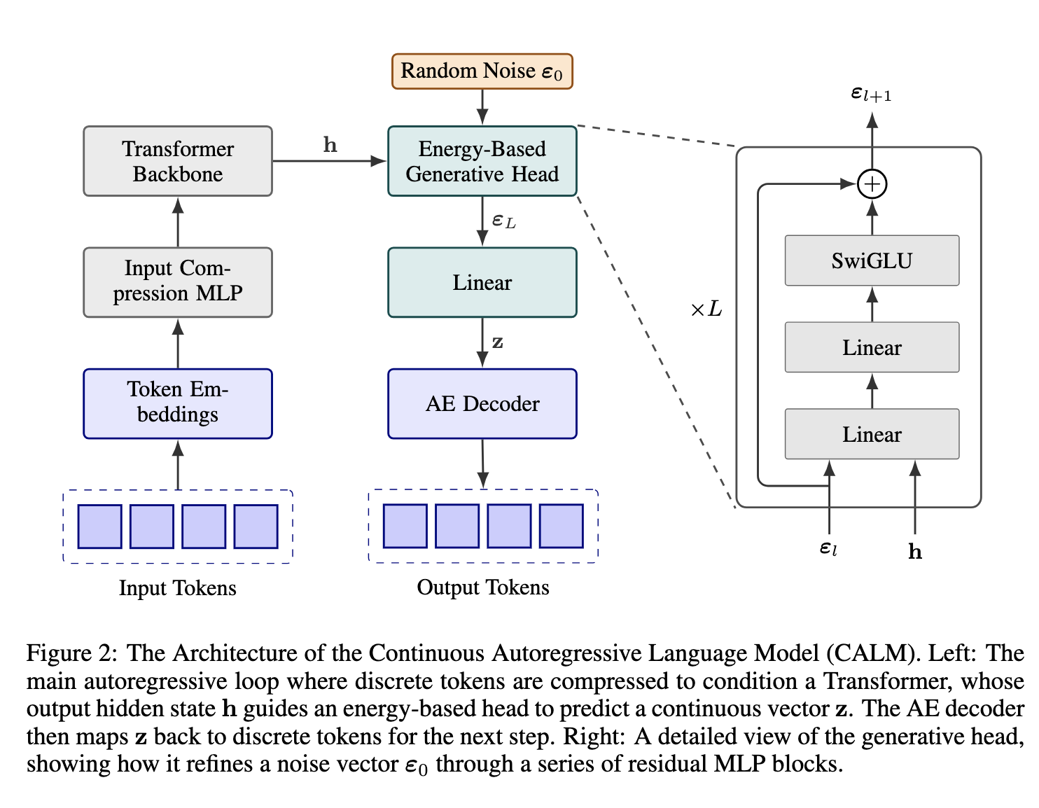
A Continuous Autoregressive Language Model (CALM) restructures the language modeling pipeline into three cooperating modules:
(1) a latent autoencoder that defines the continuous representational space,
(2) an autoregressive transformer that predicts future latents, and
(3) an energy-based generative head that evaluates and refines predictions without discrete normalization.
Together, these modules form a self-contained generative system that evolves through a continuous latent trajectory and reconstructs coherent text segments at each step.
Architectural Overview
A traditional autoregressive model factorizes text as:
\(p(x_{1:T}) = \prod_{t=1}^{T} p(x_t \mid x_{<t}),\)
where each $p(x_t \mid x_{<t})$ is a categorical distribution computed via a softmax head on top of a transformer.
In contrast, CALM introduces an intermediate latent space $\mathcal{Z} \subset \mathbb{R}^{d_z}$ and performs autoregression in that space:
\(p(z_{1:M}) = \prod_{m=1}^{M} p(z_m \mid z_{<m}),\)
with $M < T$ and each latent $z_m$ encoding multiple tokens’ worth of semantics.
The generation pipeline is therefore:
- Encoding: map input text $x_{1:T}$ to latents $z_{1:M}$ via $E_\phi$.
- Autoregression: predict $\hat{z}{t}$ from $z{<t}$ using a transformer $F_\theta$.
- Decoding: map predicted latents $\hat{z}{1:M}$ back to text via $D\psi$.
The result is a model that predicts in a continuous domain but produces discrete outputs through reconstruction, preserving the interpretability of natural text.
The Latent Autoencoder
The autoencoder defines the embedding and reconstruction functions: \(z_{1:M} = E_\phi(x_{1:T}), \quad \hat{x}_{1:T} = D_\psi(z_{1:M}).\)
Encoder $E_\phi$
- Typically a transformer or convolutional network operating over token embeddings.
- Aggregates local contexts into fixed-size latent vectors $z_m \in \mathbb{R}^{d_z}$.
- The compression ratio $K = T/M$ controls how many tokens each latent summarizes.
Mathematically, each latent is obtained through a context-dependent pooling operation: \(z_m = \text{Pool}(h_{mK - K + 1:mK}),\) where $h_t$ are intermediate hidden states of the encoder. The pooling may be attention-based, weighted by token importance or content entropy.
Decoder $D_\psi$
- A transformer or lightweight autoregressive model conditioned on latent vectors.
- Expands each $z_m$ into $K$ tokens using cross-attention from token queries to latent keys.
- Ensures smooth, context-aware reconstruction, preserving local syntactic order while maintaining global coherence.
The autoencoder is trained to minimize a reconstruction loss and optionally a KL divergence toward a latent prior $p(z)$, creating a stable, regularized latent space with roughly isotropic geometry.
Continuous Autoregressive Transformer
Once the latent space is established, CALM replaces the discrete token transformer with an autoregressive transformer over latents.
Given $z_{<t}$, the transformer produces a contextual state:
\(h_t = F_\theta(z_{<t}),\)
which summarizes the preceding latent sequence.
Instead of projecting $h_t$ to a softmax over tokens, it produces either:
- A predicted vector $\hat{z}_t = W_p h_t$, or
- A distributional representation via an energy function $E_\theta(z_t, z_{<t})$.
This architecture retains the attention-based structure of standard transformers:
- Self-attention layers model dependencies between latent vectors, capturing long-range coherence.
- Feedforward layers refine latent transitions, acting as nonlinear dynamical updates.
- Positional encodings are adapted to latent timescales rather than token indices — enabling continuous interpolation across semantic intervals.
Because $M < T$, the sequence length during autoregression is shorter, reducing computational cost per generation step. Each transformer layer processes semantic units instead of individual tokens.
Energy-Based Generative Head
At the output, CALM discards the softmax layer used for discrete prediction.
Instead, it introduces an energy-based head that measures compatibility between a context and a candidate latent continuation.
For a predicted hidden state $h_t$, the energy function is:
\(E_\theta(z_t, z_{<t}) = \frac{1}{2} \| W_e h_t - z_t \|_2^2,\)
where $W_e$ is a learnable projection matrix.
This energy is low when $z_t$ lies near the model’s expected continuation and high otherwise.
During training, the model minimizes energy for true pairs $(z_t, z_{<t})$ and maximizes it for negatives $(\tilde{z}t, z{<t})$, shaping a continuous energy field that guides prediction.
This replaces categorical probability normalization with relative energy ranking.
The output no longer represents discrete likelihoods but geometric distances in latent space, consistent with continuous semantics.
Forward Pass Summary
Putting these pieces together, a CALM forward pass proceeds as follows:
-
Input encoding:
Convert tokenized input $x_{1:T}$ into embeddings and compress via $E_\phi$: \(z_{1:M} = E_\phi(x_{1:T}).\) -
Autoregressive prediction:
For each step $t$, compute: \(\hat{z}_t = F_\theta(z_{<t}), \quad E_\theta(z_t, z_{<t}) = \frac{1}{2}\|W_e h_t - z_t\|^2.\) -
Loss computation:
Combine reconstruction and energy-based terms: \(\mathcal{L}_{\text{total}} = \mathcal{L}_{\text{rec}} + \lambda \, \mathcal{L}_{\text{energy}},\) where $\lambda$ balances latent reconstruction with predictive accuracy. -
Decoding:
At inference, predict a latent sequence $\hat{z}_{1:M}$ autoregressively, then decode: \(\hat{x}_{1:T} = D_\psi(\hat{z}_{1:M}).\)
Each autoregressive step produces multiple tokens of text via the decoder, achieving higher semantic throughput and faster generation.
Architectural Comparison: CALM vs. Discrete LLM
| Component | Standard LLM | CALM |
|---|---|---|
| Representation | Discrete tokens $x_t$ | Continuous latents $z_t \in \mathbb{R}^{d_z}$ |
| Context modeling | Transformer over tokens | Transformer over latents |
| Output layer | Softmax over vocabulary | Energy-based projection in latent space |
| Objective | Cross-entropy / NLL | Likelihood-free (energy or distance-based) |
| Sequence length | $T$ | $M = T / K$ |
| Generation | One token per step | Multiple tokens per step |
| Evaluation | Perplexity | Energy distance / Brier score / reconstruction fidelity |
This architecture unifies the interpretability of autoregression with the expressivity of continuous generative modeling. The transformer backbone remains unchanged — CALM simply redefines its representational substrate and output semantics.
Computational Considerations
While CALM increases per-step computation slightly due to the autoencoder and energy head, it reduces total generation cost by an order of magnitude through compression:
- Autoregressive steps drop by a factor of $K$.
- Each latent prediction covers multiple tokens.
- The softmax layer — typically the most expensive component — is removed entirely.
Memory footprint also decreases: the output projection matrix shrinks from $V \times d$ to $d_z \times d$, which is often 10–100× smaller since $V$ can exceed $10^5$ while $d_z$ is usually a few hundred.
Training is more stable than it might appear, because the reconstruction loss grounds the system in discrete text space, while the energy head shapes smooth transitions in latent space.
In summary, CALM preserves the transformer’s architecture while transforming its semantics.
The encoder–decoder pair defines a continuous language manifold, the autoregressive transformer models trajectories within it, and the energy head governs coherence without discrete normalization.
Together, they constitute a scalable architecture that generalizes next-token prediction into next-state evolution — enabling efficient, multi-token, continuous language generation.
Modeling in Continuous Space
Once text is represented as a sequence of continuous latent vectors, language modeling becomes a problem of predicting the next vector in a sequence of real-valued variables rather than the next discrete token. This reformulation changes the geometry of the generative process, the form of the loss function, and even the interpretation of “probability” in language modeling.
Next-Vector Prediction vs. Next-Token Prediction
In discrete autoregression, each step predicts a categorical distribution over a vocabulary. The model learns to output one of $V$ possible symbols, and the training signal is a log-likelihood derived from the cross-entropy between the predicted and true token distributions.
In CALM, each step predicts a continuous latent vector:
\[\hat{z}_{t} = f_\theta(z_{<t})\]where $f_\theta$ is a neural function, typically a transformer operating on the sequence of previous latent vectors. The target $z_t$ is a dense, real-valued vector in $\mathbb{R}^{d_z}$. The model no longer outputs probabilities over discrete outcomes but rather a point (or distribution) in continuous space.
This change is not cosmetic; it alters the entire modeling regime. Instead of asking “what is the most likely next token?”, the model asks “what is the next point on the semantic manifold that best continues the latent trajectory?”. The process resembles predicting the next frame in a continuous dynamical system rather than drawing from a categorical vocabulary.
The Failure of Likelihood in Continuous Latent Models
In discrete settings, maximizing likelihood is straightforward because the categorical probability distribution is normalized. For continuous latent spaces, defining an explicit density $p(z_t \mid z_{<t})$ is both unnecessary and often intractable.
To see why, consider that the autoencoder’s encoder $E_\phi$ maps text sequences to a latent distribution $q_\phi(z \mid x)$, which is typically complex, non-Gaussian, and implicitly defined by the network architecture. Its exact density is unknown. Modeling $p_\theta(z_t \mid z_{<t})$ with an explicit likelihood would require computing or approximating this density, which is computationally prohibitive and theoretically fragile.
Moreover, the true goal is not density estimation but distributional matching: the predicted latent $\hat{z}_t$ should fall within the same manifold region as the ground-truth $z_t$. This leads to likelihood-free learning, where the model is trained using distance- or energy-based objectives rather than normalized probabilities.
Likelihood-Free Learning
In a likelihood-free framework, the model learns to approximate the conditional distribution of latent vectors without explicitly normalizing it. Instead of minimizing $-\log p_\theta(z_t \mid z_{<t})$, we minimize a divergence between predicted and true samples.
The simplest case uses a regression-style loss, such as mean squared error:
\[\mathcal{L}_{\text{MSE}} = \| \hat{z}_t - z_t \|_2^2,\]but this ignores uncertainty: it treats all deviations equally and collapses the distribution to its mean. A more general approach uses an energy function $E_\theta(z_t, z_{<t})$, which assigns low energy to plausible continuations and higher energy to implausible ones. This leads to a loss based on proper scoring rules, which ensure that the model’s predictions are statistically consistent with the data distribution even without an explicit likelihood.
Energy-Based Objectives
An energy-based model defines an unnormalized density through an energy function:
\[p_\theta(z_t \mid z_{<t}) \propto \exp(-E_\theta(z_t, z_{<t})).\]The training objective encourages the model to assign lower energy to true latent vectors than to samples drawn from other regions of the latent space. Conceptually, the energy surface defines the “semantic potential field” over which latent dynamics evolve.
Training can use contrastive or score-matching objectives. For example, a contrastive loss takes the form:
\[\mathcal{L}_{\text{energy}} = \mathbb{E}_{z_t \sim q_\phi} \left[ E_\theta(z_t, z_{<t}) \right] + \lambda \, \mathbb{E}_{\tilde{z}_t \sim p_{\text{neg}}} \left[ \exp(-E_\theta(\tilde{z}_t, z_{<t})) \right],\]where $p_{\text{neg}}$ is a distribution of negative (implausible) samples. This objective pushes down the energy of true latents and raises the energy of negatives, shaping a structured semantic landscape where each context $z_{<t}$ defines a local basin of meaning.
Unlike a softmax, this energy formulation requires no explicit normalization over the latent space; the model learns implicitly by relative ranking. This makes it robust to the complex, non-uniform densities typical of encoded text.
Geometry of Continuous Prediction
The dynamics of continuous autoregression can be viewed geometrically. The sequence of latent vectors $(z_1, z_2, \dots, z_T)$ forms a smooth curve on the data manifold in $\mathbb{R}^{d_z}$. The model $f_\theta$ learns a function that predicts the tangent or local continuation of this curve, effectively modeling the trajectory of semantic evolution.
This interpretation connects CALM to dynamical systems and manifold learning. Each new latent prediction $\hat{z}_t$ extends the semantic trajectory according to the model’s learned flow field, ensuring that successive latent vectors remain within the manifold region corresponding to plausible text.
Unlike discrete token sequences, where transitions jump between categorical states, CALM trajectories evolve continuously in vector space, preserving differentiability and allowing gradient-based optimization across long horizons.
Learning and Regularization of the Predictive Function
Because CALM models predict continuous vectors, overfitting and instability can occur if the predictive function $f_\theta$ learns to extrapolate into regions of latent space not supported by the encoder distribution. Regularization strategies include:
- Latent prior matching: penalizing deviations from the latent prior $p(z)$ ensures predictions stay within a valid semantic region.
- Noise injection: injecting small Gaussian noise into predicted latents during training improves robustness and mimics real-world uncertainty.
- Energy margin constraints: enforcing a margin between positive and negative energy samples stabilizes learning and prevents the model from collapsing to trivial minima.
These techniques collectively maintain a structured latent trajectory that stays near the natural language manifold, allowing the decoder to reconstruct coherent text even from predicted latents.
Energy-Based Generative Modeling and Evaluation
In continuous autoregression, the model predicts a dense latent vector at each step rather than a probability over tokens. This invalidates traditional likelihood-based evaluation metrics such as perplexity, which depend on normalized categorical probabilities. CALM instead adopts an energy-based interpretation, where prediction quality is assessed via proper scoring rules defined on continuous spaces.
From Likelihoods to Energies
Recall that an energy-based model defines an unnormalized conditional distribution
\[p_\theta(z_t \mid z_{<t}) \propto \exp(-E_\theta(z_t, z_{<t})),\]where $E_\theta$ is an energy function parameterized by the model. The energy $E_\theta(z_t, z_{<t})$ acts as a scalar compatibility measure between the context $z_{<t}$ and the candidate continuation $z_t$ — lower energy corresponds to higher plausibility.
Unlike the softmax, this formulation does not require a normalization term over $\mathbb{R}^{d_z}$, which is intractable in high dimensions. Instead, training encourages the energy assigned to true continuations to be lower than that of negative samples.
This formulation captures continuous plausibility: it is no longer about selecting a discrete token, but about evaluating where in semantic space the model expects the next latent to fall. The energy surface thus encodes a smooth landscape over latent space, with valleys corresponding to coherent continuations.
Proper Scoring Rules in Continuous Spaces
Because CALM does not operate on explicit probabilities, we need a way to measure whether its predictions are well-calibrated. This is done through strictly proper scoring rules, which define consistent losses for probabilistic or energy-based predictors without requiring normalized likelihoods.
A scoring rule $S(p, y)$ is strictly proper if it is minimized only when $p$ equals the true conditional distribution of $y$. For discrete autoregressive models, cross-entropy is the canonical proper scoring rule. In CALM, we use continuous analogues such as the Brier score and energy distance.
The Brier score measures the squared deviation between the predicted and true outcomes, generalized here to vector-valued latent variables:
\[\mathcal{L}_{\text{Brier}} = \mathbb{E} \left[ \| f_\theta(z_{<t}) - z_t \|_2^2 \right].\]Although simple, it serves as a proper scoring rule under Gaussian assumptions and penalizes misalignment in the latent geometry.
More advanced formulations introduce kernelized energy distances, defining a discrepancy between predicted and true latent distributions that respects the manifold structure of the latent space. These can be written as:
\[\mathcal{L}_{\text{ED}} = \mathbb{E}\|z_t - \hat{z}_t\| - \frac{1}{2}\mathbb{E}\|z_t - z_t'\| - \frac{1}{2}\mathbb{E}\|\hat{z}_t - \hat{z}_t'\|,\]where primes denote independent samples. The energy distance vanishes if and only if the two distributions match.
The Energy Transformer
In CALM, the Energy Transformer replaces the softmax projection head of standard language models. It takes the contextual representation of previous latents and produces an energy score over the candidate next latent.
Formally, if $h_t = F_\theta(z_{<t})$ denotes the transformer output summarizing the prior latents, then the energy of a candidate continuation $z_t$ is:
\[E_\theta(z_t, z_{<t}) = \frac{1}{2} \| W_e h_t - z_t \|_2^2,\]where $W_e$ is a learned projection matrix aligning hidden states with latent embeddings. This quadratic energy defines a potential well centered around the model’s predicted next vector. The model minimizes this energy for ground-truth $z_t$ and maximizes it for negatives, sculpting a predictive field in latent space.
The key difference from a softmax head is that no categorical normalization occurs. The model learns directly in Euclidean or manifold geometry rather than over a discrete simplex. This makes generation continuous and differentiable with respect to latent coordinates.
Evaluating CALM: Beyond Perplexity
In traditional autoregressive models, evaluation uses perplexity, defined as the exponential of the average negative log-likelihood. For CALM, this metric is meaningless because $p(z_t \mid z_{<t})$ is not explicitly normalized. Instead, evaluation relies on energy-based metrics that measure alignment between predicted and encoded latents.
Common evaluation strategies include:
-
Latent reconstruction error:
Mean squared error or cosine similarity between predicted and true latents over the validation set.
This measures how well the autoregressive model captures latent dynamics. -
Decoder-based evaluation:
Decode both predicted latents $\hat{z}{1:M}$ and true latents $z{1:M}$ back into text via the decoder $D_\psi$, and compute metrics like BLEU, ROUGE, or semantic similarity.
This quantifies how accurately the continuous model reproduces linguistic content. -
Brier-based calibration:
Adapt the Brier score to measure consistency of predictions over latent uncertainty. This assesses whether predicted energies correlate with reconstruction likelihoods.
Through these metrics, CALM can be evaluated in ways that respect its continuous nature while maintaining correspondence to language-level fidelity.
Generative Sampling in Latent Space
Generation in CALM follows an iterative latent prediction process:
- Initialize with a latent prefix $z_{1:k}$ obtained by encoding a prompt.
- Predict the next latent $\hat{z}{k+1} = f\theta(z_{1:k})$.
- Optionally sample around $\hat{z}_{k+1}$ using a temperature-controlled perturbation.
- Decode the sequence of latents into text via $D_\psi(\hat{z}_{1:M})$.
Unlike token-by-token sampling, this process generates multiple words per step, as each latent corresponds to a text segment. Sampling can be smoothed or stochastic depending on the desired diversity.
To inject diversity analogous to temperature scaling in discrete models, CALM applies likelihood-free temperature sampling. Given an energy $E_\theta(z_t, z_{<t})$, we define the sampling distribution:
\[p_T(z_t \mid z_{<t}) \propto \exp\!\left(-\frac{E_\theta(z_t, z_{<t})}{T}\right),\]where $T$ controls the exploration-exploitation tradeoff. A lower $T$ focuses on high-probability (low-energy) regions, while higher $T$ encourages diversity in generated text.
Connection to Speculative and Amortized Decoding
Speculative decoding in discrete models uses a small “draft” model to propose multiple token candidates that a larger model then verifies. CALM extends this intuition to the continuous regime. Because each latent encodes multiple tokens, a single predicted latent can be viewed as a continuous speculative proposal that encapsulates many possible token sequences within its decoded manifold region.
Instead of verifying each discrete proposal independently, the energy function implicitly measures the compatibility of the entire proposed latent with the semantic trajectory. This generalizes speculative decoding into a differentiable amortized generation process: multiple future tokens are proposed and semantically validated in a single continuous step.
Training and Empirical Insights
Training a Continuous Autoregressive Language Model involves two tightly coupled processes:
(1) constructing a robust text-to-latent autoencoder, and
(2) learning a continuous predictive model that evolves latent trajectories according to linguistic dynamics.
Each process imposes its own challenges in optimization, regularization, and evaluation.
The Two-Stage Training Pipeline
CALM training proceeds in two major stages, corresponding to learning the representation space and the temporal dynamics.
- Stage 1 — Latent Space Formation (Autoencoder Training)
The autoencoder is trained on large-scale text data to compress and reconstruct sequences:- The encoder $E_\phi$ learns to map variable-length token spans to latent vectors $z_i \in \mathbb{R}^{d_z}$.
- The decoder $D_\psi$ reconstructs text from latents, enforcing high-fidelity regeneration.
- Training employs reconstruction loss plus regularizers such as KL divergence or noise perturbation penalties.
Once trained, $E_\phi$ and $D_\psi$ define a fixed, smooth manifold where latent variables correspond to semantically meaningful text regions.
- Stage 2 — Continuous Autoregressive Modeling
The transformer $F_\theta$ is trained to predict the next latent given previous latents: \(\hat{z}_t = F_\theta(z_{<t})\) The training objective can be mean-squared error, energy distance, or other likelihood-free criteria.
Importantly, gradients propagate through latent predictions only — the decoder is not used during autoregressive training, ensuring the model learns semantic progression rather than token-level copying.
This decomposition stabilizes learning: the autoencoder defines the geometry, and the autoregressive model learns the temporal field that evolves within it.
Regularization Strategies for Stable Latent Dynamics
Predicting in continuous space introduces new pathologies absent in discrete settings. Because there is no categorical normalization, latent predictions can drift, collapse, or leave the manifold region supported by the encoder. CALM mitigates these through targeted regularization:
-
Energy Margin Constraints
During training, the model minimizes energy for true latents while enforcing a margin between positive and negative samples: \(E_\theta(z_t, z_{<t}) + \gamma < E_\theta(\tilde{z}_t, z_{<t}),\) where $\tilde{z}_t$ are negatives sampled from nearby latent states and $\gamma$ is a fixed margin.
This encourages a well-structured potential landscape where valid continuations form low-energy basins separated by clear semantic boundaries. -
Noise Perturbation and Denoising
Adding Gaussian noise $\epsilon \sim \mathcal{N}(0, \sigma^2 I)$ to latent inputs or predictions during training forces the model to learn denoising behavior: \(\hat{z}_t = F_\theta(z_{<t} + \epsilon).\) This improves generalization and ensures robustness to small errors accumulated during long sequence generation. -
Latent Prior Regularization
A prior $p(z)$ (typically isotropic Gaussian) constrains the marginal distribution of encoded and predicted latents.
Minimizing divergence $\text{KL}(q_\phi(z) | p(z))$ encourages compact, normalized latent space geometry that prevents uncontrolled drift.
Together, these techniques maintain continuity and coherence in the latent sequence, making long-horizon prediction feasible without catastrophic accumulation of small errors.
Multi-Token Prediction and Effective Compression
One of the most striking empirical observations in CALM is its ability to predict multiple tokens per step without explicit instruction to do so. This arises naturally from the compression factor $K = T/M$, where $K$ tokens are represented by one latent vector.
When decoding, the model produces text segments corresponding to predicted latents:
\(\hat{x}_{t:t+K-1} = D_\psi(\hat{z}_t).\)
If the autoencoder is trained to reconstruct $K$-token chunks, then each autoregressive step of CALM effectively emits $K$ tokens’ worth of semantics in a single prediction.
This yields an O(K) speedup in generation relative to discrete autoregression, with minimal loss in linguistic coherence.
Empirical results show that even with modest compression ratios (e.g., $K=3$ or $4$), CALM achieves comparable text quality while reducing sequential computation by up to 75%. Higher compression is possible, but with diminishing returns: extreme compression blurs syntactic precision and reduces text diversity.
Efficiency Gains: Bandwidth and Throughput
The advantage of continuous autoregression can be quantified in terms of semantic bandwidth — the rate of meaningful information transmitted per generative step. For discrete models, this bandwidth is capped at $\log_2 V$ bits per step. For CALM, each step transmits a vector of dimension $d_z$ with continuous precision, giving an upper bound of approximately $d_z \log_2 (1/\epsilon)$ bits, where $\epsilon$ is floating-point granularity.
Even accounting for noise and redundancy, this represents a large increase in theoretical throughput.
Practically, this means that a continuous model can express more semantic information per forward pass, enabling shorter sequences and lower latency for equivalent text content.
Latency and FLOPs analysis confirms that the majority of runtime in large language models comes from repeated transformer decoding. Reducing autoregressive steps by a factor of $K$ directly multiplies decoding speed without increasing model size — a major computational win.
Empirical Stability and Quality
Qualitative experiments show that CALM retains coherence and fluency across multi-sentence continuations, even when predicting 4–8 tokens per latent. The reconstructed text exhibits:
- Semantic continuity: generated sentences maintain logical consistency with prior context.
- Stylistic smoothness: transitions between predicted segments are fluid, reflecting continuous latent trajectories.
- Compositional recall: factual or structural elements from earlier context persist across latent boundaries.
Ablations reveal several key sensitivities:
- KL weight in the autoencoder controls the smoothness of latent space; too low and the model memorizes, too high and reconstruction degrades.
- Latent dimensionality $d_z$ trades off expressivity and generalization; around 1/8th of transformer hidden size yields strong results.
- Noise scale during training improves robustness but excessive noise destabilizes the decoder.
Overall, continuous autoregression matches or exceeds the linguistic quality of discrete autoregression at a fraction of the computational cost.
Theoretical Implications
From a theoretical standpoint, CALM bridges the gap between discrete symbolic modeling and continuous dynamical systems. The latent sequence behaves like a trajectory on a manifold $\mathcal{M} \subset \mathbb{R}^{d_z}$, and the autoregressive transformer defines a vector field over this manifold:
\[z_{t+1} = F_\theta(z_t) + \eta_t,\]where $\eta_t$ represents residual uncertainty. This turns language generation into a differentiable flow through semantic space, with smooth, learnable dynamics rather than discrete jumps.
The model thus provides a continuous-time interpretation of language evolution — each latent step integrates meaning along a low-dimensional manifold.
Broader Implications and Theoretical Connections
Continuous Autoregressive Language Models (CALMs) represent more than an optimization of decoding efficiency — they redefine how linguistic structure is represented and generated.
By replacing discrete token-level transitions with continuous latent evolution, CALM merges ideas from autoregressive modeling, energy-based learning, and continuous dynamical systems. This section situates CALM within that conceptual landscape.
The End of Discrete Bottlenecks
Traditional autoregressive models treat language as a discrete stochastic process. The next token is sampled from a categorical distribution, and the model learns to approximate the conditional entropy of that process.
This framing has worked remarkably well but imposes a structural bottleneck: it assumes that all meaningful linguistic information can be discretized into atomic, mutually exclusive categories.
CALM breaks this assumption.
By emitting continuous latent vectors, it treats language not as a sequence of discrete decisions, but as a trajectory through a continuous semantic field.
Each step represents a localized movement in meaning space, allowing far richer expressivity per generative step.
This fundamentally changes the notion of “next token prediction”: rather than selecting one symbol from a finite set, the model predicts an infinitesimal displacement in semantic coordinates.
The discrete symbols we observe in text are no longer the primary modeling targets — they are projections of a deeper continuous process.
Relationship to Diffusion and Flow Matching Models
Although CALM is autoregressive rather than generative-from-noise, its mathematical structure shares deep similarities with diffusion and flow matching paradigms.
Diffusion models define a stochastic trajectory in data space, gradually denoising from pure noise to a clean sample.
Flow matching models define a deterministic trajectory governed by an ODE that transports samples along the data manifold.
CALM can be viewed as an autoregressive flow on latent space: \(z_{t+1} = F_\theta(z_t) + \eta_t,\) where $\eta_t$ is stochastic noise capturing uncertainty or linguistic diversity.
Conceptually:
- Diffusion models traverse data space from noise to data.
- Flow matching models traverse from prior to data in continuous time.
- CALM traverses within the data manifold in discrete steps, evolving semantics in a temporally autoregressive fashion.
In all cases, the underlying principle is identical: learning a differentiable transformation that preserves the geometry of a manifold while generating new samples consistent with that structure.
CALM’s innovation lies in embedding this idea into the autoregressive formulation — combining the temporal compositionality of language with the smoothness of continuous flows.
Connection to Energy-Based and Score-Based Models
Energy-based models (EBMs) assign scalar energies to configurations, shaping a potential landscape whose minima correspond to valid data points.
CALM’s predictive mechanism is precisely an energy function $E_\theta(z_t, z_{<t})$, defining how compatible a proposed continuation $z_t$ is with its context.
Thus, CALM can be understood as a conditional EBM over latent trajectories.
This connection clarifies its generative semantics: rather than directly sampling from an explicit distribution, CALM draws from regions of low energy, where encoded latents naturally reside.
The autoregressive transformer learns to navigate these basins sequentially, predicting new latents that remain on the manifold of linguistic plausibility.
Score-based models, which learn the gradient of the log-density $\nabla_z \log p(z)$, can be seen as infinitesimal versions of this process — predicting small vector displacements that increase data likelihood.
CALM’s vector predictions are discrete-time analogues of these continuous gradient flows, driven by an implicit energy function learned through data alignment.
Speculative and Amortized Decoding Revisited
Speculative decoding in traditional LLMs accelerates generation by drafting multiple candidate tokens and verifying them with a larger model.
In CALM, this paradigm emerges naturally and continuously: each latent prediction acts as a continuous speculative proposal representing a region of plausible text continuations.
The decoder $D_\psi$ implicitly “verifies” these proposals by reconstructing coherent text only if the latent lies on the semantic manifold.
This constitutes amortized speculative decoding: the draft and verification steps collapse into one differentiable operation.
The model no longer needs to test multiple discrete hypotheses — it predicts directly within the space of valid semantic representations.
This is a profound efficiency gain: speculative reasoning becomes a built-in geometric property of the model rather than a procedural algorithm.
The Geometry of Language
The introduction of continuous latent dynamics transforms our interpretation of linguistic structure.
Language, in this view, is not a symbolic string but a trajectory through a high-dimensional semantic manifold.
Tokens correspond to projections of this continuous curve onto discrete coordinates — a quantization of meaning for communication, not an inherent property of cognition or computation.
The autoregressive transformer in CALM thus models the vector field of language flow: how ideas, syntax, and context evolve over time in a differentiable space.
Each step integrates this field, producing the next semantic state, which the decoder later renders into observable text.
This geometric framing aligns with long-standing intuitions in cognitive science and information theory: that linguistic meaning evolves continuously even though we observe it as discrete tokens.
CALM provides the first large-scale generative architecture to operationalize this view directly.
Toward Unified Continuous Generative Models
CALM sits at the intersection of three paradigms:
| Paradigm | Data Representation | Generative Mechanism | Example |
|---|---|---|---|
| Autoregressive | Discrete | Token-by-token factorization | GPT-style LLMs |
| Diffusion / Flow | Continuous | Denoising or ODE integration | Stable Diffusion, Flow Matching |
| Continuous Autoregression (CALM) | Continuous (latent) | Autoregressive latent evolution | CALM family |
Each paradigm models a different axis of the same underlying process — the evolution of structured information across time or noise scales.
CALM unifies them by showing that autoregression itself can be made continuous: prediction, sampling, and evaluation all become smooth, differentiable operations in latent space.
This reframing hints at a larger future direction: unified generative fields that blend autoregressive structure, diffusion-like smoothness, and energy-based consistency within a single continuous modeling framework.
Outlook and Open Questions
The CALM formulation opens several avenues for further exploration:
- Temporal resolution: can we train models that operate at variable semantic timescales, dynamically adjusting compression $K$ as needed?
- Cross-modal extension: continuous autoregression could generalize naturally to video, audio, or multimodal data, where semantics evolve smoothly over time.
- Hybrid architectures: combining discrete control (for symbolic reasoning) with continuous evolution (for semantic fluidity).
- Theoretical grounding: formalizing convergence guarantees, stability of latent trajectories, and information-theoretic limits of continuous autoregression.
If successful, these directions may redefine the limits of generative modeling — moving from discrete symbol prediction to continuous understanding and synthesis.