Recommendation Systems • Eval, Metrics and Loss
- Overview
- Offline testing - Pre deployment
- Online testing - Post deployment
- Evaluate Candidate Generation
- Evaluate Scoring
- Evaluate Ranking
- Accuracy metrics
- Engagement Metrics
- Click-Through Rate (CTR)
- Average number of clicks per user
- Conversion Rate (CVR)
- Session Length
- Dwell Time
- Bounce Rate
- Hit Rate
- Average Reciprocal Hit Rate (ARHR)
- Mean Average Precision at N (mAP@N) and Mean Average Recall at N (mAR@N)
- mAP@N and mAR@N
- Normalized Discounted Cumulative Gain
- Correlation metrics
- F1 Score
- Loss
- References
Overview
- In this page, we will look at how different evaluation techniques, loss functions and metrics for recommender systems. When it comes to evaluating different types of recommender systems, the choice of metrics varies.
- For content-based filtering, similarity metrics are commonly used, while predictive and classification metrics are more relevant for collaborative filtering, depending on whether the system predicts scores or binary outcomes.
- Evaluation is essential to dissuade misalignment between the model and the user and choosing the correct metrics can help understand if your model is optimizing for the correct objective function.
- Good recommender systems are obtained by constant improvement and that comes with attention to metrics. Additionally, in practice, there may be a need to use more than one metric and in this case, calculating a weighted average of multiple metrics can be used to obtain a single overall score.
- Note that metrics in recommender systems are not just for user experience but also for creators (with metrics like Coverage) who build on the platform or for advertisers and all non-integrity violating items in the corpus should be fair game for recommendations.
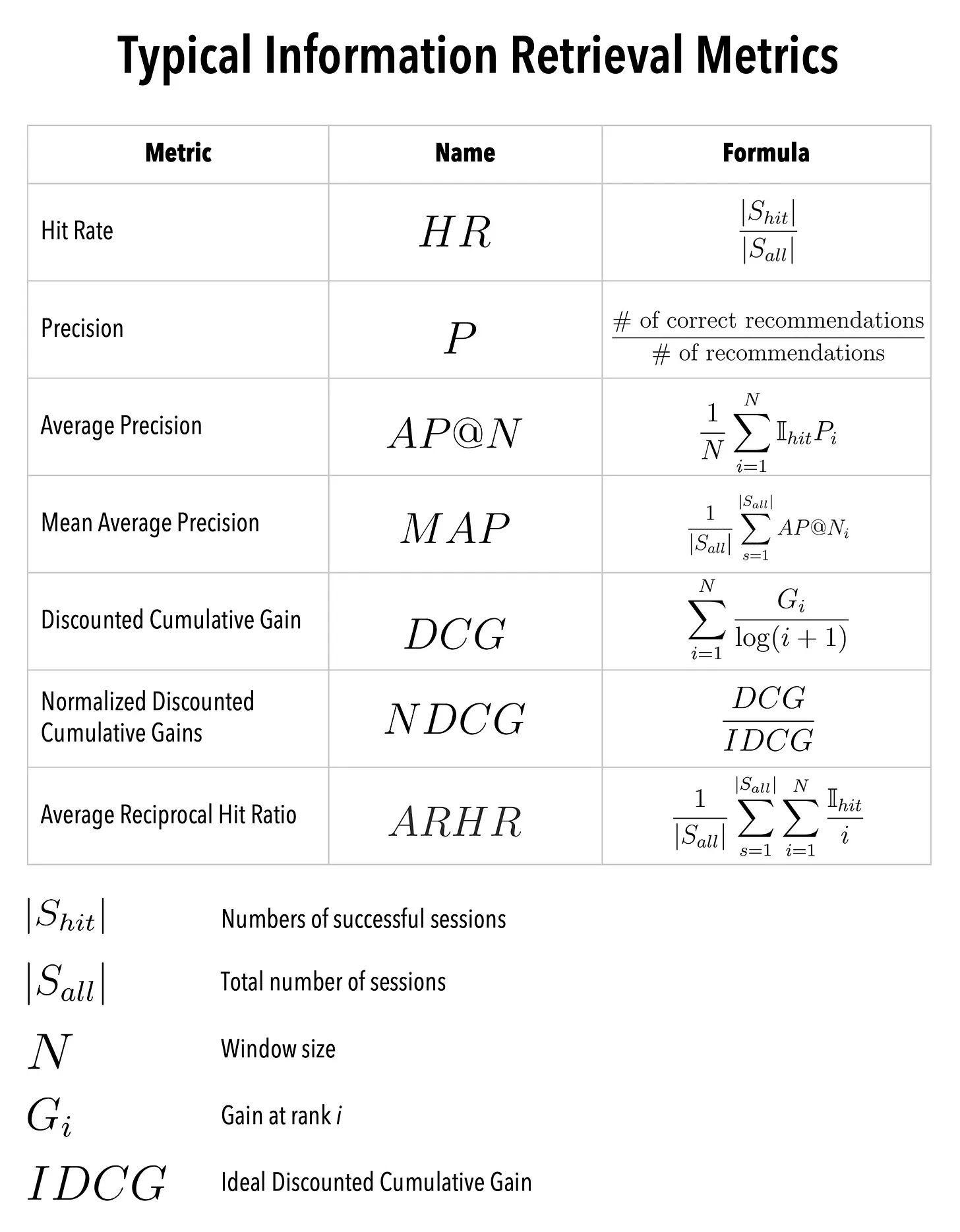
- Below (source), we can see the common and typical metrics leveraged in IR which is where recommender systems borrow their metrics from.
Offline testing - Pre deployment
- Offline testing or pre-deployment testing is an important step in evaluation recommender systems before deploying to production. The main purpose of offline testing is to estimate the model’s performance using historical data and benchmark it against other candidate models.
- Offline evaluations generally follow a train-test evaluation procedure which entails:
- Data Preparation: The first step is to prepare and select the appropriate historical data set and partition it into training and test sets.
- Model Training: Next, we train the model using the training set which can involve choosing the right algorithms, tuning hyperparameters and selecting eval metrics.
- Model Evaluation: Once the model is trained, it’s evaluated using the test set and the metrics used here depend on the business use case.
- Model Selection: Based on the evaluation, the best performing model is selected for deployment.
Online testing - Post deployment
- Online testing for recommender systems is the process of evaluating the system and it’s performance in a live environment. Once the pre-deployment/offline testing looks good, we test it on a small fraction of real user visits.
- The goal of online testing is to ensure that the system works as expected in a real-world environment with respect to the objective function and metrics. This can be achieved by A/B or Bucket testing and we will delve into it in detail below.
A/B Testing or Bucket Testing
- A/B testing involves running two versions of a model simultaneously and assigning users to either the control or the treatment bucket by leveraging a hash function.
- The users in the treatment bucket will receive recommendations from the new model while the control bucket users will continue to receive recommendations from the existing model.
- The performance of each model is measured with metrics based on the business need, for example, CTR can be used if the objective is to maximize clicks.
- A/B testing can be used for any step in the recommendation system lifecycle, including candidate generation, scoring or ranking.
- It can be used to identify the best configuration of hyperparameters, such as regularization strength, learning rate, and batch size. In addition, A/B testing can be used to test different recommendation strategies, such as popularity-based, personalized, and diversity-based, and to identify the most effective strategy for different user segments and business contexts.
Evaluate Candidate Generation
- Candidate generation involves selecting a set of items from a large pool of items that are relevant to a particular user. The candidate generation phase plays a crucial role in recommender systems, especially for large-scale systems with many items and users, as it helps to reduce the search space and improve the efficiency of the recommendation process.
- It is essential to evaluate candidate generation as it affects the overall performance of the recommender system. Poor candidate generation can lead to a recommendation process that is either too narrow or too broad, resulting in a poor user experience. Additionally, it can lead to inefficient use of resources, as irrelevant items may be included in the recommendation process, requiring more computational power and time.
- There are a few metrics that can help evaluate candidate generation:
- Diversity: Diversity measures the degree to which recommended items cover different aspects of the user’s preferences. One way to calculate diversity is to compute the average pairwise dissimilarity between recommended items.
-
Example, say you have 3 categories of items the user likes, if the user has interacted with item 1 only in this session, this would mean the session is not diverse.
\[\text { CosineSimilarity }(i, j)=\frac{\text { count (users who bought } i \text { and } j \text { ) }}{\sqrt{\text { count (users who bought } i)} \times \sqrt{\text { count (users who bought } j \text { ) }}}\] -
Novelty: Novelty measures the degree to which recommended items are dissimilar to those already seen by the user.
\[\operatorname{Novelty}(i)=1-\frac{\text { count(users recommended } i)}{\text { count(users who have not interacted with } i \text { ) }}\] - Serendipity: This is the ability of the system to recommend items that a user might not have thought of but would find interesting or useful. Serendipity is an important aspect of recommendation quality as it can help users discover new and interesting items that they might not have found otherwise.
Evaluate Scoring
- Scoring is the measure of how the model’s prediction was rated by the user. The recommender will assign a score or weight to each item in the candidate set, based on how relevant it is to the user.
- Evaluation of scoring can be measured by taking the absolute value of the difference of the predicted and actual value: \(abs(actual - predicted)\). A few other methods are by leveraging the following metrics:
- Precision: Precision is the metric used to evaluate the accuracy of the system as it measures the number of relevant items that were recommended divided by the total number of recommended items.
- Precision = Number of recommended items that are relevant / Total number of recommended items
- Recall: Recall is a metric that measures the percentage of relevant items that were recommended, out of all the relevant items available in the system. A higher recall score indicates that the system is able to recommend a higher proportion of relevant items. In other words, it measures how complete the system is in recommending all relevant items to the user.
- Recall = Number of recommended items that are relevant / Total number of relevant items
- Normalized Discounted Cumulative Gain (NDCG): NDCG (Normalized Discounted Cumulative Gain) is a listwise ranking metric used to evaluate the quality of a recommender system’s ranked list of recommendations.
- To understand NDCG, we first need to understand DCG (Discounted Cumulative Gain) and CG (Cumulative Gain).
- DCG: DCG is a ranking evaluation metric that measures the effectiveness of a recommendation system in generating a ranked list of recommended items for a user. It takes into account the relevance of the recommended items and their position in the list. DCG, which stands for Discounted Cumulative Gain, is a measure of the quality of the ranking of a set of items. It takes into account both the relevance of each item and its position in the ranking. The idea is that items that are ranked higher should be more relevant and contribute more to the overall quality of the ranking.
- CG: CG, which stands for Cumulative Gain, is a simpler measure that just sums up the relevance scores of the top k items in the ranking.
- Thus, NDCG, which stands for Normalized Discounted Cumulative Gain, is a normalized version of DCG that takes into account the ideal ranking, which is the ranking that maximizes the DCG. The idea is to compare the actual ranking to the ideal ranking to see how far off it is.
- Precision: Precision is the metric used to evaluate the accuracy of the system as it measures the number of relevant items that were recommended divided by the total number of recommended items.
- Note: calibration of scores is also essential in recommender systems to ensure that the predicted scores or ratings are reliable and an accurate representation of the user’s preferences. With calibration, we adjust the predicted scores to match the actual scores as there may be a gap due to many factors: data, changing business rules, etc.
- A few techniques that can be used for this are:
- Post-processing methods: These techniques adjust the predicted scores by scaling or shifting them to match the actual scores. One example of a post-processing method is Platt scaling, which uses logistic regression to transform the predicted scores into calibrated probabilities.
- Implicit feedback methods: These techniques use implicit feedback signals, such as user clicks or time spent on an item, to adjust the predicted scores. Implicit feedback methods are particularly useful when explicit ratings are sparse or unavailable.
- Regularization methods: These techniques add regularization terms to the model objective function to encourage calibration. For example, the BayesUR algorithm adds a Gaussian prior to the user/item biases to ensure that they are centered around zero.
Evaluate Ranking
- The goal of ranking is to optimize for the objective function and this can be done post deployment by using metrics such as CTR, Time Spent, etc.
- Mean reciprocal recall: Mean reciprocal rank (MRR) is a popular metric for evaluating ranking in recommender systems. It is a measure of how well the algorithm ranks the correct item in a list of recommendations.
- MRR is calculated as the average of the reciprocal rank of the first relevant item across all the users. The reciprocal rank is defined as the inverse of the rank of the first relevant item.
- Precision/Recall: Precision and Recall can also be used here as it was used in scoring.
- Click-through rate (CTR): CTR is a commonly used metric to evaluate ranking in recommenders. CTR is the ratio of the number of times a recommended item is clicked to the number of times it is shown to users. It provides an indication of how effective the recommendations are in terms of driving user engagement.
- \[TotalClicks/ TotalNumTimesItemShown\]
- However, CTR does not take into account the relevance or quality of the recommended items, and it can be biased towards popular or frequently recommended items.
- Mean reciprocal recall: Mean reciprocal rank (MRR) is a popular metric for evaluating ranking in recommender systems. It is a measure of how well the algorithm ranks the correct item in a list of recommendations.
- Now let’s take a look at some other metrics we have yet to mention.
Accuracy metrics
- Accuracy metrics are used to evaluate how well the model predicts the users preferences and help quantify the difference between predicted and actual ratings for a given set of recommendations.
Root mean squared (RMSE)
- This measures the square root of the average of the squared differences between predicted and actual ratings. It is commonly used for continuous ratings, such as those on a scale of 1 to 5.
Mean absolute error (MAE)
- This measures the average magnitude of the errors in a set of predictions, without considering their direction. It’s calculated by taking the average of the absolute differences between the predicted and actual values.
- This measures the average of the absolute differences between predicted and actual ratings. It is also commonly used for continuous ratings.
Log-likelihood
- This measures the goodness of fit of a model. It’s calculated by taking the logarithm of the likelihood function.
- This measures the logarithm of the probability that the model assigns to the observed data. It is commonly used for binary data, such as whether a user liked or disliked a particular item.
Engagement Metrics
- Engagement metrics are used to measure how much users engage with the recommended items. These metrics evaluate the effectiveness of the recommender system. Below we will look at a few common engagement metrics.
Click-Through Rate (CTR)
- CTR, as we saw earlier, measures the ratio of clicks to impressions. It is calculated by dividing the number of clicks by the number of impressions.
Average number of clicks per user
- As the name suggests, this calculates the average number of clicks per user and it builds on top of CTR. It allows more relevance as the denominator is changed with the total number of users instead of total number of clicks.
Conversion Rate (CVR)
- CVR measures the ratio of conversions to clicks. It is calculated by dividing the number of conversions by the number of clicks.
Session Length
- This measures the length of a user session. It is calculated by subtracting the start time from the end time of a session.
Dwell Time
- Dwell time is the measures the amount of time a user spends on a particular item. It is calculated by subtracting the time when the user stops engaging with an item from the time when the user starts engaging with it.
Bounce Rate
- Here, we measure the percentage of users who leave a page after viewing only one item. It is calculated by dividing the number of single-page sessions by the total number of sessions. \(Bounce Rate = Single-Page Sessions / Total Sessions\)
Hit Rate
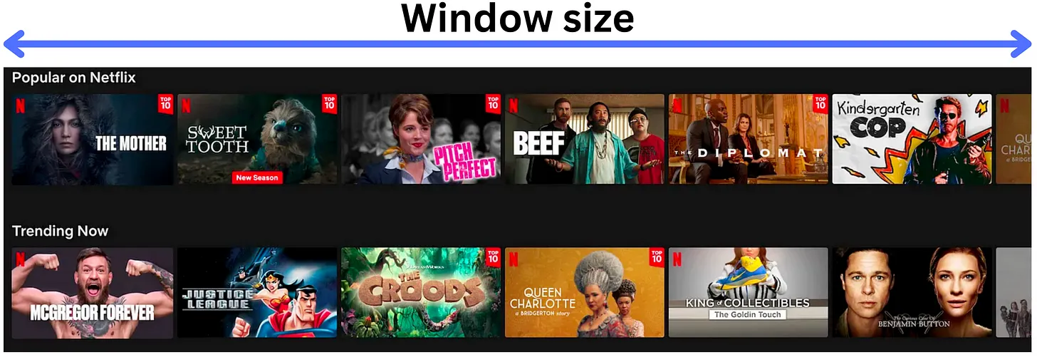
- Hit rate is concerned with the fact that out of the recommended lists, how many users watched a movie in that visible window? The window size here is custom to each product, for example for Netflix, it would be the screen size.
\(Hit Rate = Number of users that clicked within the window / Total Number of users presented with the Recommendations\)
- Below (source), we can see the window size of a screen.
Average Reciprocal Hit Rate (ARHR)
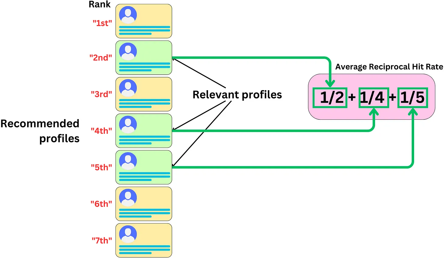
- Average Reciprocal Hit Rate (ARHR), also known as mean reciprocal rank, is a valuable metric to assess the performance of recommender systems when explicit relevance labels are not available. In such cases, the system relies on implicit signals, such as user clicks or interactions, to gauge the relevance of recommended items. ARHR takes into account the position of the recommended items in determining their relevance.
- To understand ARHR, let’s consider an example of Facebook friend suggestions. When presented with a list of recommended friends, users are more likely to click on a recommendation if it appears at the top of the list. Similar to NDCG, the position in the list serves as a measure of relevance. ARHR aims to answer the question:
- “How many items, discounted by their position, were considered relevant within the recommended list?”
- Formally, the Reciprocal Hit Rate (RHR) is calculated for each user by summing the reciprocals of the positions of the clicked items within the recommendation list. For instance, if the 3rd item in the list was clicked, its reciprocal would be 1/3. The RHR for a user is the sum of these reciprocals for all the clicked items.
- ARHR is obtained by averaging the RHR values across all users to provide an overall measure of the system’s performance. It indicates the average effectiveness of the recommender system in presenting relevant items at higher positions within the recommendation list.
- By incorporating the position of clicked items and considering the average across users, ARHR provides insights into the proportion of relevant items within the recommended list, giving more weight to those appearing at higher positions. A higher ARHR signifies that the recommender system is better at presenting relevant items prominently, resulting in improved user engagement and satisfaction.

Mean Average Precision at N (mAP@N) and Mean Average Recall at N (mAR@N)
- If the size of the window changes per device, we may want to consider all possible window options with the most relevant videos to be at the top.
- In order to do so, we will need to penalize the metrics if the most relevant videos are too far down the list. Let’s start looking at these metrics by first looking at just Precision and Recall.
Precision
-
Precision, as we saw earlier, measures how many relevant items there were in the total items that were recommended.
-
Below (source), we can see Precision illustrated.
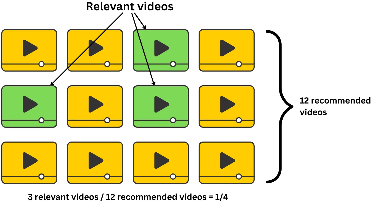 \(Precision = # of relevant items in recommendation/size of recommendation\)
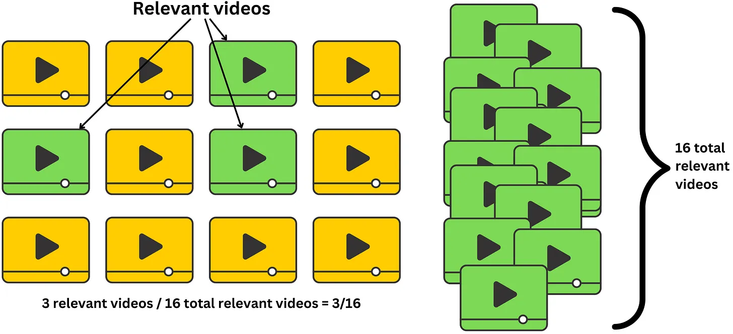
Recall
- Recall measures how many relevant items were recommended out of the total relevant items present. \(Recall = # of relevant items/ # total relevant items\)
- Below (source), we can see Recall illustrated.
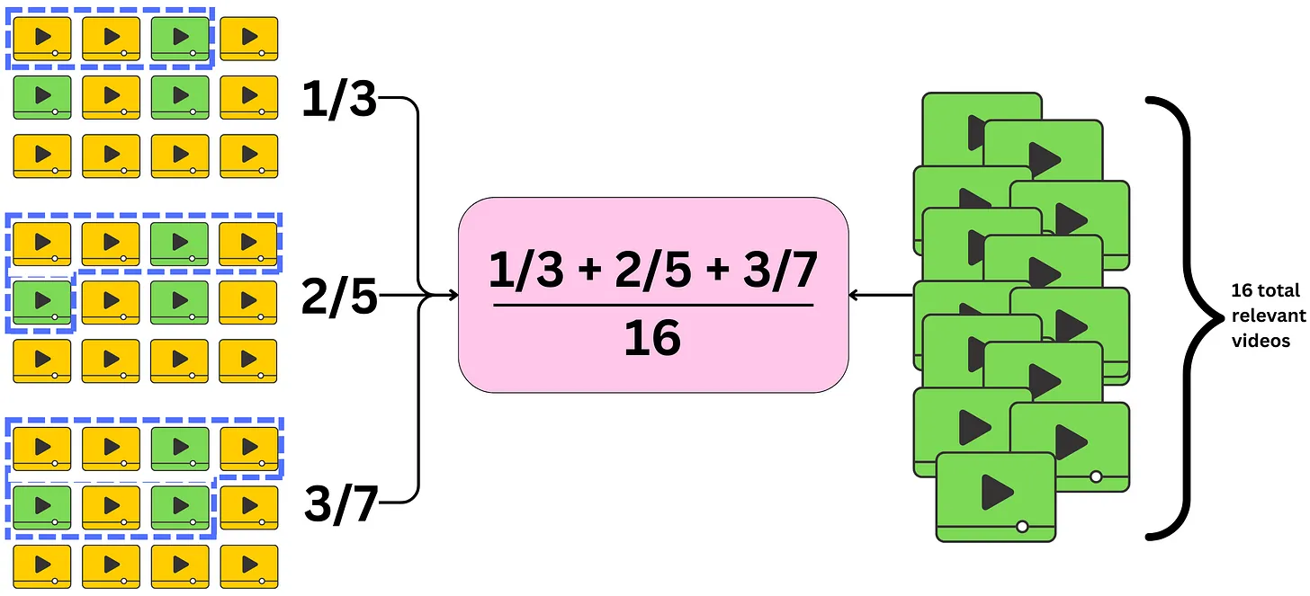
Average Precision at N (AP@N)
- Since precision and recall do not account for how far down the list relevant recommendations are, we can leverage average precision to take care of that.
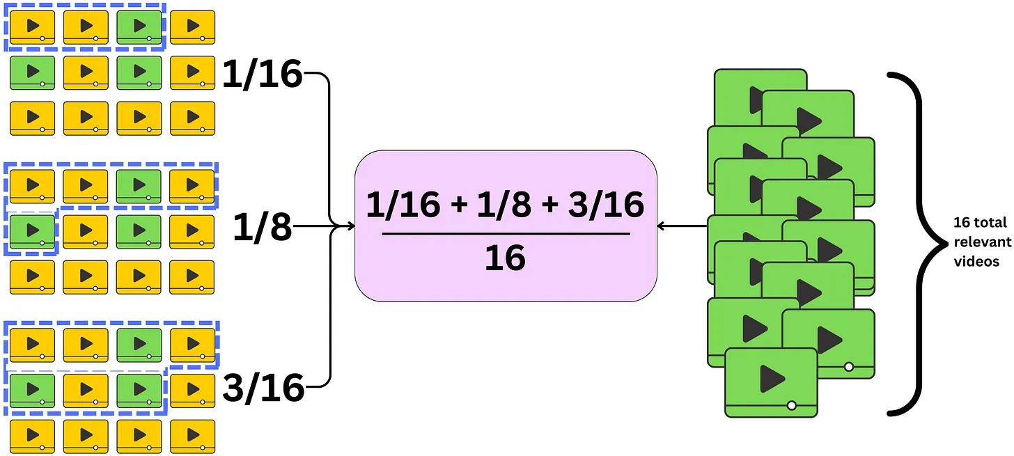
- Average precision measures the precision for any window size as seen in the images below (source).
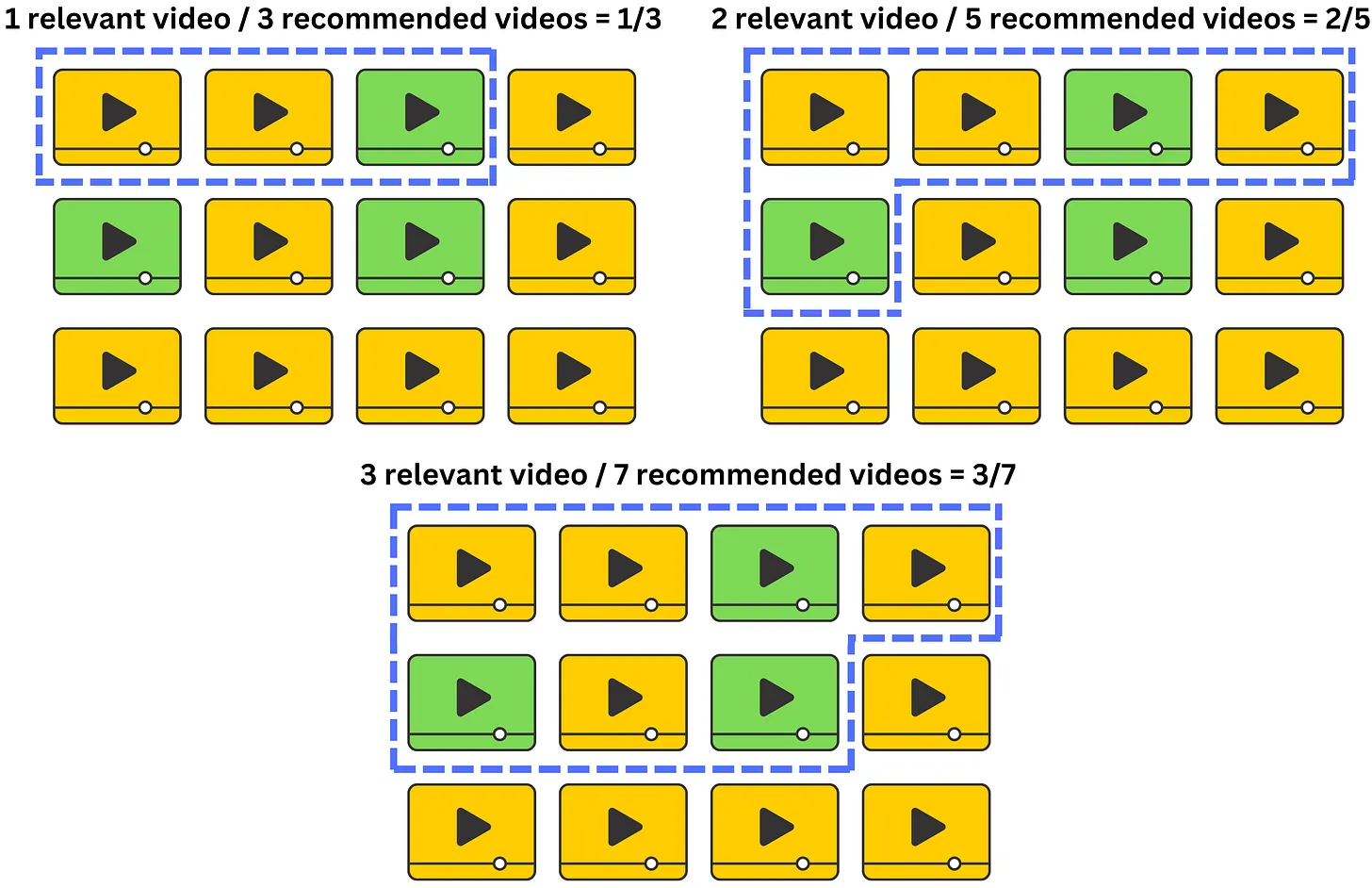
- We only include the precision in the sum if the item is relevant for that window size and we average those precisions and normalize them by the number of relevant videos.
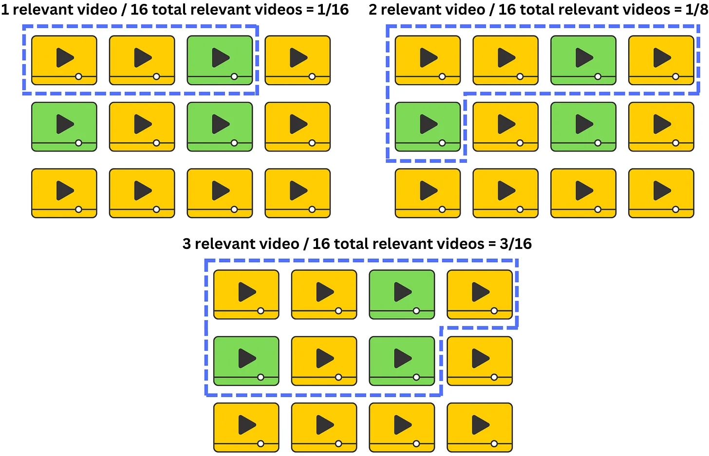
Average Recall at N (AR@N)
- Similarly, AR@N is used to calculate the average recall of a given window. The images below (source) show how AR@N will average those recalls and normalize by the number of relevant videos.
mAP@N and mAR@N
- Now let’s zoom back out to mAP@N and mAR@N.
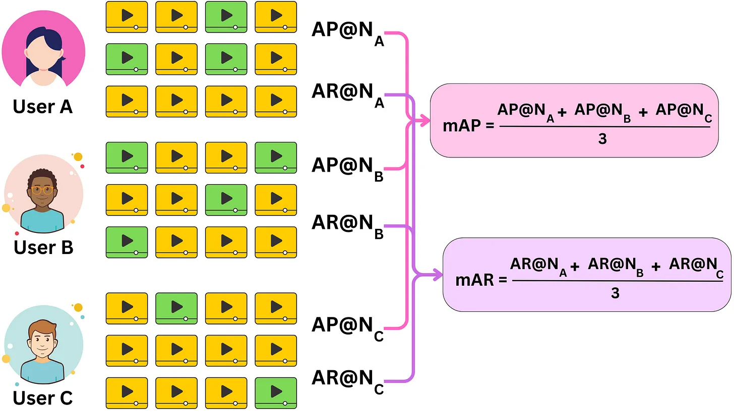
- In the context of the Mean Average Precision (MAP) metric, the term “average” encompasses the calculation of average precision across different window sizes, while “mean” pertains to the average precision computed across all users for whom the recommender system generated recommendations.
- Average across different window sizes: MAP takes into account various window sizes, which represent different cut-off points within the recommendation list. It calculates the average precision at each window size and then determines the overall average across these different window sizes. This allows for a comprehensive evaluation of the recommender system’s performance at different positions within the recommendation list.
- Mean across all users: For each user who received recommendations, the precision at each window size is calculated, and then these precision values are averaged to obtain the mean precision for that particular user. The mean precision is computed for all users who were presented with recommendations by the system. Finally, the mean of these mean precision values across all users is determined, resulting in the Mean Average Precision.
- By considering both the average precision across window sizes and the mean precision across users, MAP provides an aggregated measure of the recommender system’s performance. It captures the ability of the system to recommend relevant items at various positions in the list and provides a holistic evaluation across the entire user population.
- MAP is commonly used in information retrieval and recommender system evaluation, particularly in scenarios where the position of recommended items is crucial, such as search engine result ranking or personalized recommendation lists. \(MAP = (Sum of Average Precision for all users) / Total Number of Users\)
- In the case of the Mean Average Recall (MAR) metric, the term “average” refers to the calculation of average recall across different window sizes, while “mean” denotes the average recall computed across all users for whom the recommender system generated recommendations.
- Average across different window sizes: MAR takes into consideration various window sizes, representing different cut-off points within the recommendation list. It calculates the recall at each window size and then determines the overall average across these different window sizes. This enables a comprehensive evaluation of the recommender system’s ability to capture relevant items at different positions within the recommendation list.
- Mean across all users: For each user who received recommendations, the recall at each window size is calculated, and these recall values are averaged to obtain the mean recall for that particular user. The mean recall is computed for all users who were presented with recommendations by the system. Finally, the mean of these mean recall values across all users is determined, resulting in the Mean Average Recall.
- By considering both the average recall across window sizes and the mean recall across users, MAR provides an aggregated measure of the recommender system’s performance. It captures the system’s capability to recommend a diverse range of relevant items at various positions in the recommendation list, and it offers a holistic evaluation across the entire user population.
- MAR is commonly used in information retrieval and recommender system evaluation, particularly in scenarios where capturing relevant items throughout the recommendation list is important. It complements metrics like MAP and can provide valuable insights into the overall recall performance of the system. \(MAR = (Sum of Average Recall for all users) / Total Number of Users\)
Normalized Discounted Cumulative Gain
- Let’s take a deeper look at NDCG.
- We often need to know which items are more relevant than others, even if all the items present are relevant.

- This is because we want the most relevant items at the top of the list and to do so, occasionally, industry will hire human labelers to rate the results, for example, provided from a search query.
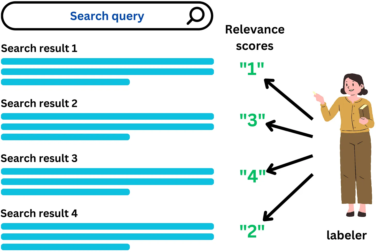
- NDCG is a widely used evaluation metric in information retrieval and recommender systems. Unlike binary metrics that only consider relevance as either relevant or not relevant, NDCG takes into account the relevance of items on a continuous spectrum.
- Let’s dive a bit deeper and break NDCG down to smaller components.
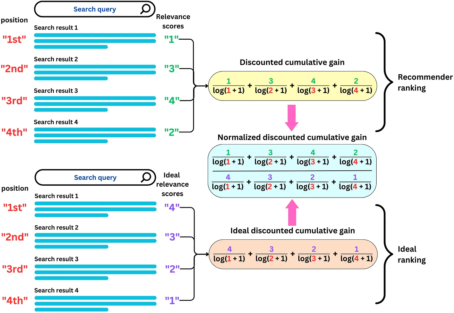
- The calculation of Discounted Cumulative Gain (DCG) is influenced by the specific values assigned to relevance labels. Even with clear guidelines, different labelers may interpret and assign relevance scores differently, leading to variations in DCG values. To address this issue and facilitate meaningful comparisons, normalization is applied to standardize DCG scores by the highest achievable value. This normalization is achieved through the concept of Ideal Discounted Cumulative Gain (IDCG).
- IDCG represents the DCG score that would be attained with an ideal ordering of the recommended items. It serves as a benchmark against which the actual DCG values can be compared and normalized. By defining the DCG of the ideal ordering as IDCG, we establish a reference point for the highest achievable relevance accumulation in the recommended list.
- The Normalized Discounted Cumulative Gain (NDCG) is derived by dividing the DCG score by the IDCG value:
- This division ensures that the NDCG values are standardized and comparable across different recommendation scenarios. NDCG provides a normalized measure of the quality of recommendations, where 1 represents the ideal ordering and indicates the highest level of relevance.
- It is important to note that when relevance scores are all positive, NDCG falls within the range of [0, 1]. A value of 1 signifies that the recommendation list follows the ideal ordering, maximizing the relevance accumulation. Conversely, lower NDCG values indicate a less optimal ordering of recommendations, with a decreasing level of relevance.
- By employing NDCG, recommender systems can evaluate their performance consistently across diverse datasets and labeler variations. NDCG facilitates the comparison of different recommendation algorithms, parameter settings, or system enhancements by providing a normalized metric that accounts for variations in relevance scores and promotes fair evaluation practices.
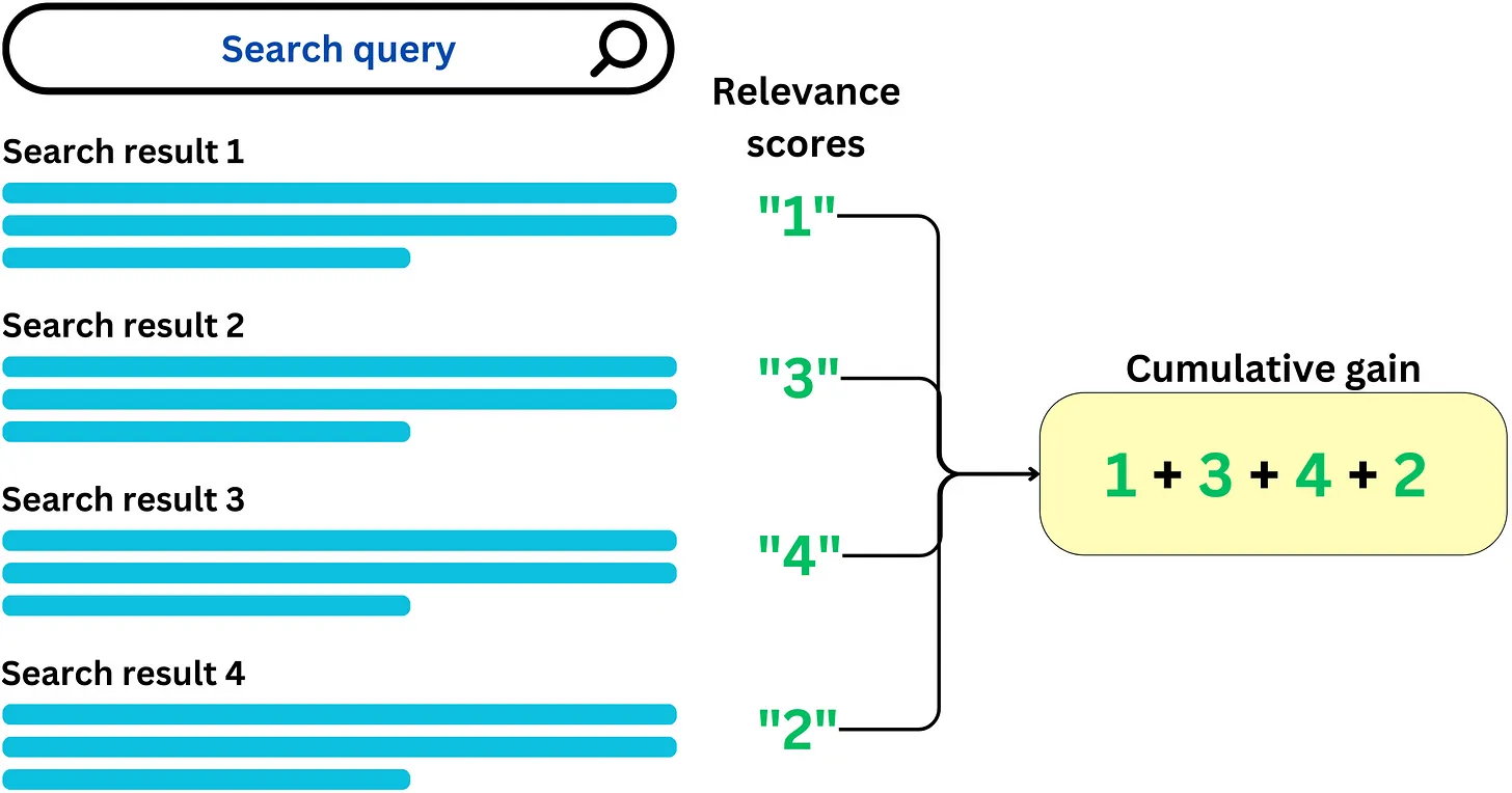
Cumulative gain (CG)
\[C G=\sum_{i=1}^N \text { relevance score } \text { sct }_i\]- Relevance labels play a crucial role in evaluating the quality of recommendations in recommender systems. By utilizing these labels, various metrics can be computed to assess the effectiveness of the recommendation process. One such metric is Cumulative Gain (CG), which aims to quantify the total relevance contained within the recommended list.
- The primary question that CG metric answers is: “How much relevance is present in the recommended list?”
- To obtain a quantitative answer to this question, we sum up the relevance scores assigned to the recommended items by the labeler. The relevance scores can be based on user feedback, ratings, or any other form of relevance measurement. However, it’s important to establish a cutoff window size, denoted by N, to ensure that we consider a finite number of elements in the recommended list.
- By setting the window size N, we restrict the calculation to a specific number of items in the recommendation list. This prevents the addition of an infinite number of elements, making the evaluation process feasible and practical.
- The cumulative gain metric allows us to measure the overall relevance accumulated in the recommended list. A higher cumulative gain indicates a greater amount of relevance captured by the recommendations, while a lower cumulative gain suggests a lack of relevant items in the list.
Discounted cumulative gain (DCG)
\(C G=\sum_{i=1}^N \text { relevance score } \text { sct }_i\)
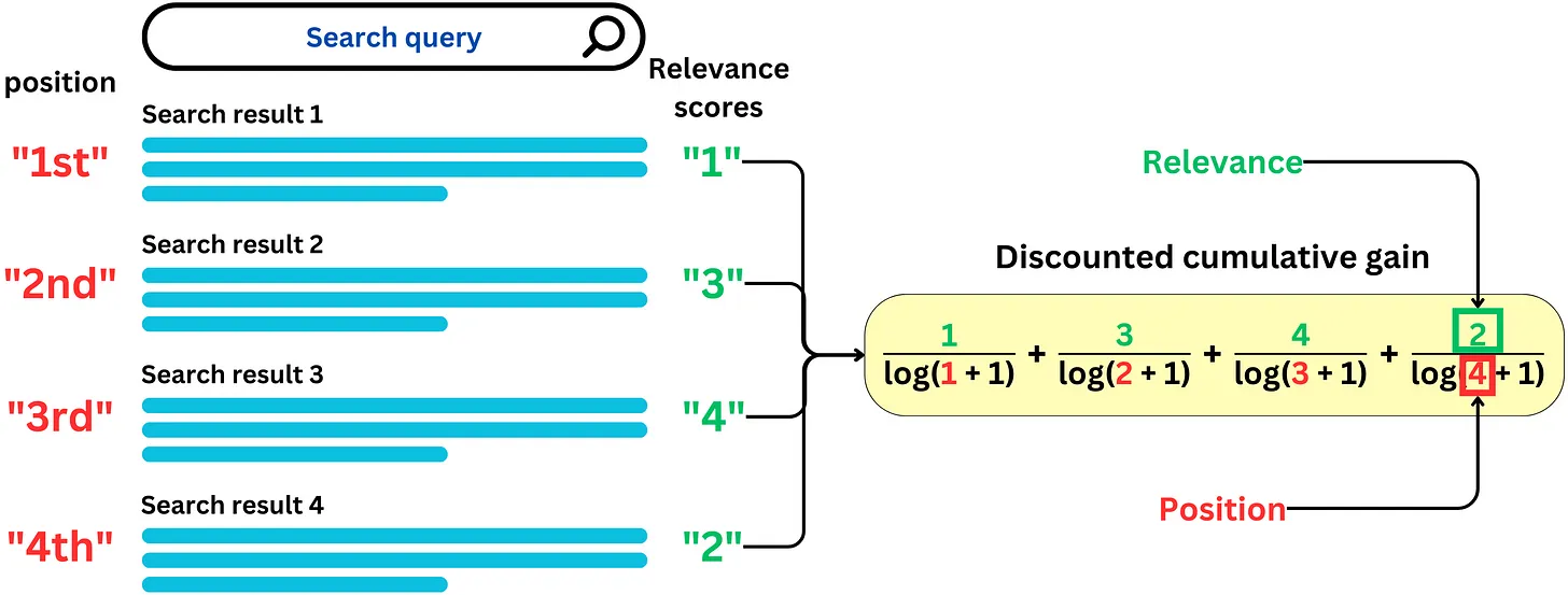
- While Cumulative Gain (CG) provides a measure of the total relevance in a recommended list, it disregards the crucial aspect of the position or ranking of search results. In other words, CG treats all items equally, regardless of their order, which is problematic since we aim to prioritize the most relevant items at the top of the list. This is where Discounted Cumulative Gain (DCG) comes into play.
- DCG addresses the limitation of CG by incorporating the position of search results in the computation. It achieves this by applying a discount to the relevance scores based on their position within the recommendation list. The idea is to assign higher weights to items at the top of the list, reflecting the intuition that users are more likely to examine and interact with the items presented first.
- Typically, the discounting factor used in DCG follows a logarithmic function. This means that as the position of an item decreases, the relevance score is discounted at a decreasing rate. In other words, the relevance score of an item at a higher position carries more weight than an item at a lower position, reflecting the diminishing importance of items as we move down the list.
Correlation metrics
- Correlation metrics can be used to evaluate the performance and effectiveness of the recommendation algorithms. These correlation measures assess the relationship between the predicted rankings or ratings provided by the recommender system and the actual user preferences or feedback. They help in understanding the accuracy and consistency of the recommendations generated by the system.
Kendall rank correlation coefficient
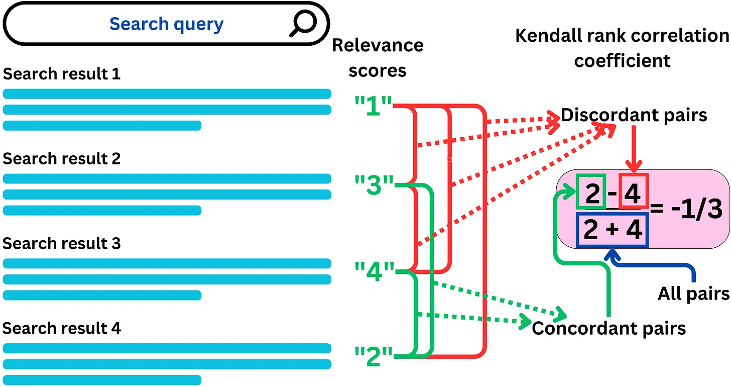
- Kendall rank correlation is well-suited for recommender systems when dealing with ranked or ordinal data, such as user ratings or preferences. It quantifies the similarity between the predicted rankings and the true rankings of items. A higher Kendall rank correlation indicates that the recommender system can successfully capture the relative order of user preferences.
Pearson Correlation
- Although Pearson correlation is primarily applicable to continuous variables, it can still be employed in recommender systems to evaluate the relationship between predicted ratings and actual ratings. It measures the linear association between the predicted and true ratings. However, it is important to note that Pearson correlation might not capture non-linear relationships, which can be common in recommender systems.
Spearman Correlation
- Similar to Kendall rank correlation, Spearman correlation is useful for evaluating recommender systems with ranked or ordinal data. It assesses the monotonic relationship between the predicted rankings and the true rankings. A higher Spearman correlation indicates a stronger monotonic relationship between the recommended and actual rankings.
F1 Score
- For binary classification problems, achieving a balance between precision and recall is often desirable. Precision measures the proportion of correctly predicted positive instances out of all predicted positive instances, while recall measures the proportion of correctly predicted positive instances out of all actual positive instances. The F1 score is a metric that combines precision and recall into a single value, capturing the balance between them.
- However, when it comes to recommender systems, the F1 score may not be the most appropriate metric to evaluate performance. In recommender systems, the focus is on providing relevant recommendations rather than making binary predictions. The trade-off between precision and recall is different in this context.
- In recommender systems, if we reduce the number of recommended items (N), precision tends to increase while recall decreases. This is because the system becomes more confident about the top-ranked items, which are more likely to be relevant. The density of relevant items among the top recommendations increases, resulting in higher precision. However, since fewer items are being recommended overall, some relevant items may be missed, leading to a decrease in recall.
- On the other hand, when we increase N and include more items in the recommendation list, precision tends to decrease while recall increases. This is because more relevant items may be included, but the inclusion of irrelevant items also becomes more likely, leading to a lower precision. However, with a larger recommendation list, more of the relevant items have a chance to be included, resulting in higher recall.
- Therefore, while the F1 score is a valid metric for binary classification problems, it may not be as suitable for evaluating recommender systems. Other metrics, such as precision, recall, average precision, or mean average precision, are often used to assess the performance of recommender systems more effectively, considering the specific goals and trade-offs involved in recommendation tasks.
Loss
- Loss functions are used in training recommender models to optimize their parameters, while evaluation metrics are used to measure the performance of the models on a held-out validation or test set.
- When training a recommender, loss functions can be used to minimize bias and enforce fairness and moderation. Below are some examples of loss functions that recommender systems can leverage:
- Fairness Loss: This loss function is used to enforce fairness constraints in the recommendation process. One way to define this loss is to minimize the difference in the predicted scores between different groups of users, e.g., users of different genders or races. The goal is to minimize the difference in outcomes between different groups of users, such as males and females, or people of different ethnicities. The fairness loss function can be defined in many ways, but a common approach is to use the difference in outcome between different groups as the loss function.
- Diversity Loss: This loss function is used to encourage the recommender to recommend diverse items. One way to define this loss is to maximize the distance between the predicted scores for different items.
- Margin Loss: This loss function is used to ensure that the system generates recommendations with a high level of confidence. The margin loss function works by penalizing the system for generating recommendations with low confidence scores. The goal is to maximize the margin loss while still generating high-quality recommendations.
References
- Statistical Methods for Recommender Systems by Deepak K. Agarwal and Bee-Chung Chen
- Tutorial on Fairness in Machine Learning by Ziyuan Zhong
- Recall and Precision for Recommender Systems
- Serendipity: Accuracy’s Unpopular Best Friend in Recommenders by Eugene Yan
- AIEdge Deep Dive into all the Ranking Metrics