Intro to ML Design
- Overview
- Feature Engineering
- Problem statement
- Identify metrics
- Identify requirements
- Train and evaluate model
- Design high level system
- Scale the design
- Feature Selection and Feature Engineering
- Feature hashing in tech companies
- Crossed feature
- Embedding
- How to generate/learn embedding vector?
- Embedding in tech companies
- Numeric features
- Training Pipeline
- Retraining requirements
- Inference
- Serving logics and multiple models
- Non-stationary problem
- Exploration vs. exploitation: Thompson Sampling
- Metrics evaluation
- Offline metrics
- Online metrics
- Input Pipeline
- Loading data
- Feature Stores
- Data flywheel
- Evaluate before deploy via Validation set
Overview
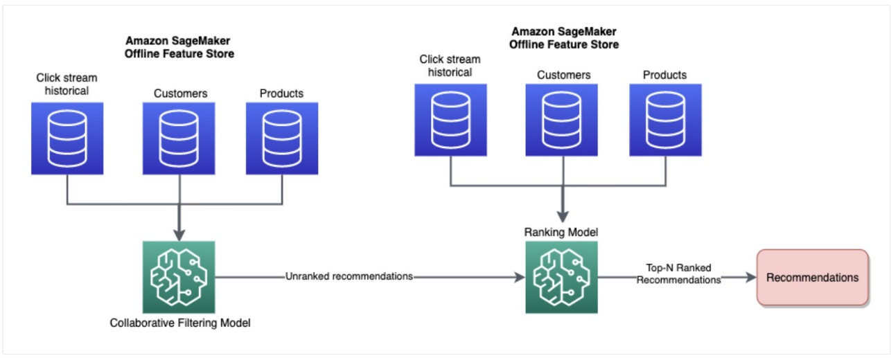
- Amazon Rec MOdel example
- Alex Xu’s non AI design: Linked here
- The standard development cycle of machine learning includes data collection, problem formulation, model creation, implementation of models, and enhancement of models.
- It is in the company’s best interest throughout the interview to gather as much information as possible about the competence of applicants in these fields.
- There are plenty of resources on how to train machine learning models and how to deploy models with different tools.
- However, there are no common guidelines for approaching machine learning system design from end to end. This was one major reason for designing this course.

- More links here
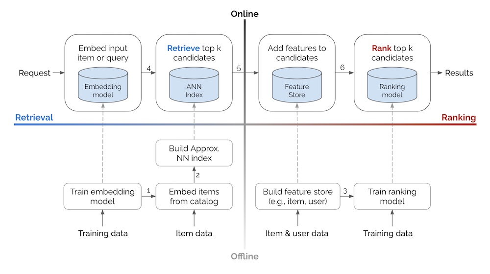
- The image below (source), does a great job at giving a holistic overview.
Feature Engineering
- Feature engineering can happen at both the candidate generation and ranking level:
- A feature store typically holds both features and associated data that are relevant for the recommendation process. Let’s break down the components of a feature store:
- Features: The primary purpose of a feature store is to store and provide access to the computed or pre-aggregated features. Features represent the characteristics, attributes, or properties of users, items, or contextual information that are used to make recommendations. These features can be numerical, categorical, or even textual representations. Examples of features in a recommender system may include user demographics, item attributes, user-item interaction history, contextual data (time, location, etc.), or derived features generated through feature engineering.
-
Metadata: Along with the features, a feature store may also store additional metadata related to the entities in the recommendation system. This metadata can include information such as unique identifiers for users and items, timestamps, user preferences, item descriptions, or any other relevant information that provides additional context or descriptive details about the entities.
-
Relationships: A feature store may also capture relationships or associations between entities in the system. For example, it may store information about user-to-user relationships (e.g., social connections), item-to-item relationships (e.g., similarity measures), or any other relationships that can be useful for recommendation purposes.
-
Indexing and Storage Information: In addition to the actual feature and metadata data, a feature store may also include indexing and storage-related information. This can include indexes or lookup tables that enable efficient retrieval of features based on user or item identifiers, storage configurations for optimized performance (e.g., partitioning, sharding), or any other relevant information for managing and accessing the feature store efficiently.
The feature store serves as a centralized repository of the relevant data and features needed for the recommendation process. It provides a unified and efficient way to access, query, and retrieve the necessary information for candidate generation, ranking, or other recommendation tasks.
It’s important to note that while a feature store holds valuable data for recommendations, it may not store the entire raw dataset or the complete historical data. Instead, it stores preprocessed, transformed, or aggregated representations of the data that are specifically designed for efficient retrieval and utilization in the recommendation pipeline.
- Retrieval Phase Features:
- User Features: These features represent characteristics and preferences of the user. They can include demographic information (age, gender, location), user profile attributes, historical behavior (purchase history, browsing history), explicit feedback (ratings, reviews), implicit feedback (clicks, view counts), or social network information.
- Item Features: These features capture the attributes and characteristics of the items. They can include item metadata (title, description, category), item attributes (price, brand, release date), textual features (keywords, tags), visual features (images, thumbnails), or audio features (for media content).
- Contextual Features: These features capture contextual information that may influence the recommendation, such as time of day, location, device type, or current user session information.
- The purpose of these features in the retrieval phase is to filter out a subset of candidate items that are potentially relevant to the user. The features are used to match the user’s preferences, characteristics, and context with the item attributes. This helps to narrow down the pool of items and retrieve a set of candidates for further ranking.
- Ranking Phase Features:
- Interaction Features: These features capture the user’s interactions with items, such as ratings, purchase history, click-through rates, or dwell time. They reflect the user’s engagement and preferences towards specific items.
- Collaborative Filtering Features: These features capture similarities or relationships between users and items based on their past interactions. They can include user-item similarity scores, user-item co-occurrence statistics, or neighborhood-based collaborative filtering measures.
- Content-Based Features: These features capture the relevance and similarity between items based on their content attributes. They can include text similarity measures, image similarity measures, or other content-based similarity metrics.
- Personalization Features: These features aim to capture personalized aspects of the recommendation, such as user-specific biases, user clusters or segments, or user-specific preferences extracted from historical data.
- In the ranking phase, these features are used to model the relevance and quality of each candidate item to the user. They help in determining the order or ranking of the items to make the final recommendations. The features are used in machine learning models or ranking algorithms to estimate the likelihood or predicted preference of the user towards each item.
Problem statement
- It’s important to state the correct problems. It is the candidates job to understand the intention of the design and why it is being optimized. It’s important to make the right assumptions and discuss them explicitly with interviewers. For example, in a LinkedIn feed design interview, the interviewer might ask broad questions:
- Design LinkedIn Feed Ranking.
- Asking questions is crucial to filling in any gaps and agreeing on goals. The candidate should begin by asking follow-up questions to clarify the problem statement. For example:
- Is the output of the feed in chronological order?
- How do we want to balance feeds versus sponsored ads, etc.?
- If we are clear on the problem statement of designing a Feed Ranking system, we can then start talking about relevant metrics like user agreements.
Identify metrics
- During the development phase, we need to quickly test model performance using offline metrics.
- You can start with the popular metrics like logloss and AUC for binary classification, or RMSE and MAPE for forecast.
Identify requirements
- Training requirements
- There are many components required to train a model from end to end. These components include the data collection, feature engineering, feature selection, and loss function. For example, if we want to design a YouTube video recommendations model, it’s natural that the user doesn’t watch a lot of recommended videos. Because of this, we have a lot of negative examples. The question is asked:
- How do we train models to handle an imbalance class?
- Once we deploy models in production, we will have feedback in real time.
- How do we monitor and make sure models don’t go stale?
- Inference requirements
- Once models are deployed, we want to run inference with low latency (<100ms) and scale our system to serve millions of users.
- How do we design inference components to provide high availability and low latency?
Train and evaluate model
- There are usually three components: feature engineering, feature selection, and models. We will use all the modern techniques for each component.
- For example, in Rental Search Ranking, we will discuss if we should use ListingID as embedding features. In Estimate Food Delivery Time, we will discuss how to handle the latitude and longitude features efficiently.
Design high level system
- In this stage, we need to think about the system components and how data flows through each of them. The goal of this section is to identify a minimal, viable design to demonstrate a working system. We need to explain why we decided to have these components and what their roles are.
- For example, when designing Video Recommendation systems, we would need two separate components: the Video Candidate Generation Service and the Ranking Model Service.
Scale the design
- In this stage, it’s crucial to understand system bottlenecks and how to address these bottlenecks. You can start by identifying:
- Which components are likely to be overloaded?
- How can we scale the overloaded components?
- Is the system good enough to serve millions of users?
- How we would handle some components becoming unavailable, etc.
Feature Selection and Feature Engineering
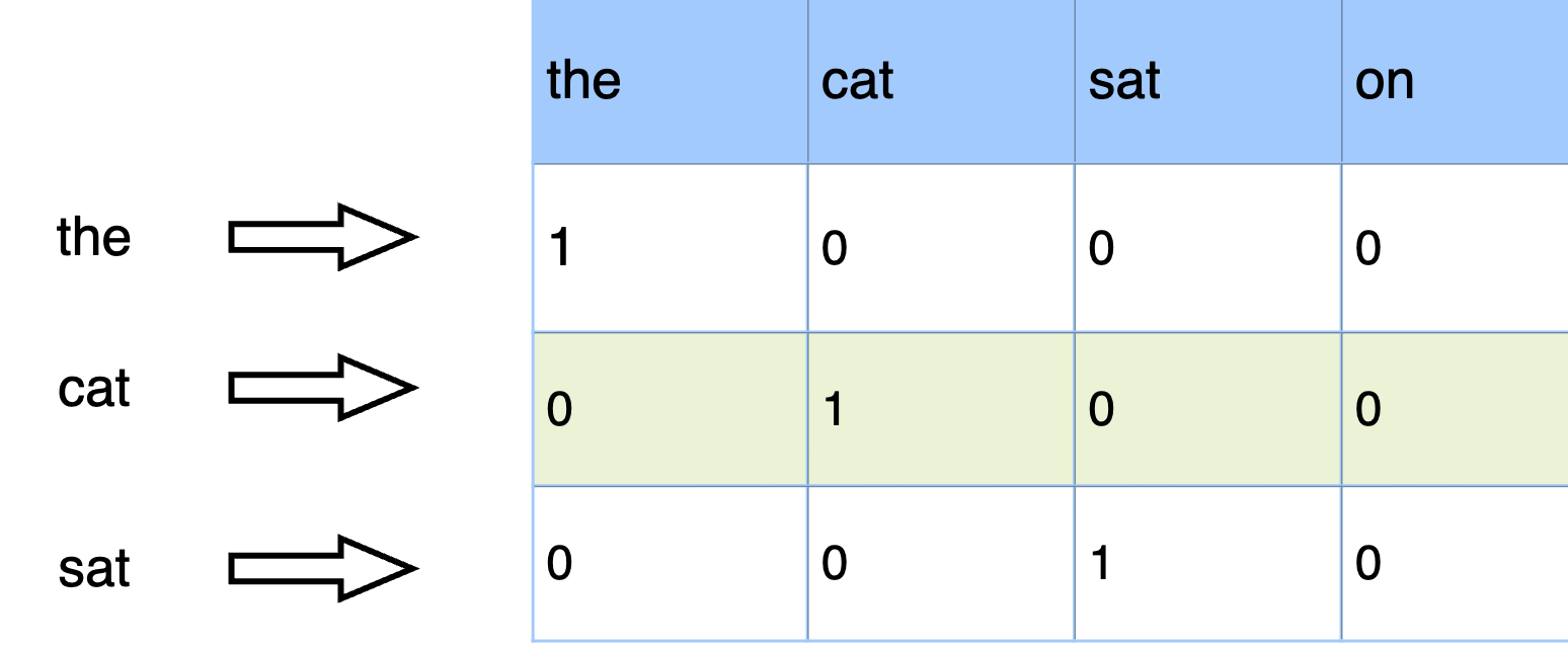
One hot encoding
- One hot encoding is a very common technique in feature engineering. It converts categorical variables into a one-hot numeric array.
- One hot encoding is very popular when you have to deal with categorical features that have medium cardinality.
In Python, there are many ways to do one hot encoding, for example, pandas.get_dummies and sklearn OneHotEncoder. pandas.get_dummies does not “remember” the encoding during training, and if testing data has new values, it can lead to inconsistent mapping.
OneHotEncoder is a Scikitlearn Transformer; therefore, you can use it consistently during training and predicting.
Common problems
- Expansive computation and high memory consumption are major problems with one hot encoding. High numbers of values will create high-dimensional feature vectors. For example, if there are one million unique values in a column, it will produce feature vectors that have a dimensionality of one million.
- One hot encoding is not suitable for Natural Language Processing tasks. Microsoft Word’s dictionary is usually large, and we can’t use one hot encoding to represent each word as the vector is too big to store in memory.
Best practices
- Depending on the application, some levels/categories that are not important, can be grouped together in the “Other” class.
- Make sure that the pipeline can handle unseen data in the test set.
One hot encoding in tech companies
- It’s not practical to use one hot encoding to handle large cardinality features, i.e., features that have hundreds or thousands of unique values. Companies like Instacart and DoorDash use more advanced techniques to handle large cardinality features.
Feature hashing
- Feature hashing, called the hashing trick, converts text data or categorical attributes with high cardinalities into a feature vector of arbitrary dimensionality.
Benefits
- Feature hashing is very useful for features that have high cardinality with hundreds and thousands of unique values. Hashing trick is a way to reduce the increase in dimension and memory by allowing multiple values to be present/encoded as the same value.
-Feature hashing example
- First, you chose the dimensionality of your feature vectors. Then, using a hash function, you convert all values of your categorical attribute (or all tokens in your collection of documents) into a number. Then you convert this number into an index of your feature vector. The process is illustrated in the diagram below.
- Below is an illustration of the hashing trick for desired dimensionality of 5 for the originality of K of values of an attributes
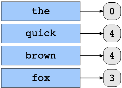
Example
- Let’s illustrate what it would look like to convert the text “The quick brown fox” into a feature vector. The values for each word in the phrase are:
the = 5
quick = 4
brown = 4
fox = 3
- Let define a hash function, h, that takes a string as input and outputs a non-negative integer. Let the desired dimensionality be 5. By applying the hash function to each word and applying the modulo of 5 to obtain the index of the word, we get:
h(the) mod 5 = 0
h(quick) mod 5 = 4
h(brown) mod 5 = 4
h(fox) mod 5 = 3
In this example:

h(the) mod 5 = 0 means that we have one word in dimension 0 of the feature vector.

h(quick) mod 5 = 4 and h(brown) mod 5 = 4 means that we have two words in dimension 4 of the feature vector.

h(fox) mod 5 = 3 means that we have one word in dimension 3 of the feature vector.

As you can see, that there are no words in dimensions 1 or 2 of the vector, so we keep them as 0.

Finally, we have the feature vector as: [1, 0, 0, 1, 2].
- As you can see, there is a collision between words “quick” and “brown.” They are both represented by dimension 4. The lower the desired dimensionality, the higher the chances of collision. To reduce the probability of collision, we can increase the desired dimensions. This is the trade-off between speed and quality of learning.
- Commonly used hash functions are MurmurHash3, Jenkins, CityHash, and MD5.
Feature hashing in tech companies
- Feature hashing is popular in many tech companies like Booking, Facebook, Yahoo, Yandex, Avazu and Criteo.
- One problem with hashing is collision. If the hash size is too small, more collisions will happen and negatively affect model performance. On the other hand, the larger the hash size, the more it will consume memory.
- Collisions also affect model performance. With high collisions, a model won’t be able to differentiate coefficients between feature values. For example, the coefficient for “User login/ User logout” might end up the same, which makes no sense.
- Depending on application, you can choose the number of bits for feature hashing that provide the correct balance between model accuracy and computing cost during model training. For example, by increasing hash size we can improve performance, but the training time will increase as well as memory consumption.
Crossed feature
- Crossed features, or conjunction, between two categorical variables of cardinality c1 and c2 is just another categorical variable of cardinality c1 × c2. If c1 and c2 are large, the conjunction feature has high cardinality, and the use of the hashing trick is even more critical in this case. Crossed feature is usually used with a hashing trick to reduce high dimensions.
- As an example, suppose we have Uber pick-up data with latitude and longitude stored in the database, and we want to predict demand at a certain location. If we just use the feature latitude for learning, the model might learn that a city block at a particular latitude is more likely to have a higher demand than others. This is similar for the feature longitude. However, a feature cross of longitude by latitude would represent a well-defined city block. Consequently, the model will learn more accurately.
- Below is Uber Pickups Map in 2015 (source Uber), Read more about different techniques in handling latitude/longitude here: Haversine distance, Manhattan distance.

- Crossed feature in tech companies
- This technique is commonly applied at many tech companies. LinkedIn uses crossed features between user location and user job title for their Job recommendation model. Airbnb also uses cross features for their Search Ranking model.
Embedding
- Feature embedding is an emerging technique that aims to transform features from the original space into a new space to support effective machine learning. The purpose of embedding is to capture semantic meaning of features; for example, similar features will be close to each other in the embedding vector space.
- Benefits
- Both one hot encoding and feature hashing can represent features in another dimension. However, these representations do not usually preserve the semantic meaning of each feature. For example, in the Word2Vector representation, embedding words into dense multidimensional representation helps to improve the prediction of the next words significantly.
- A 4-dimensional embedding below:
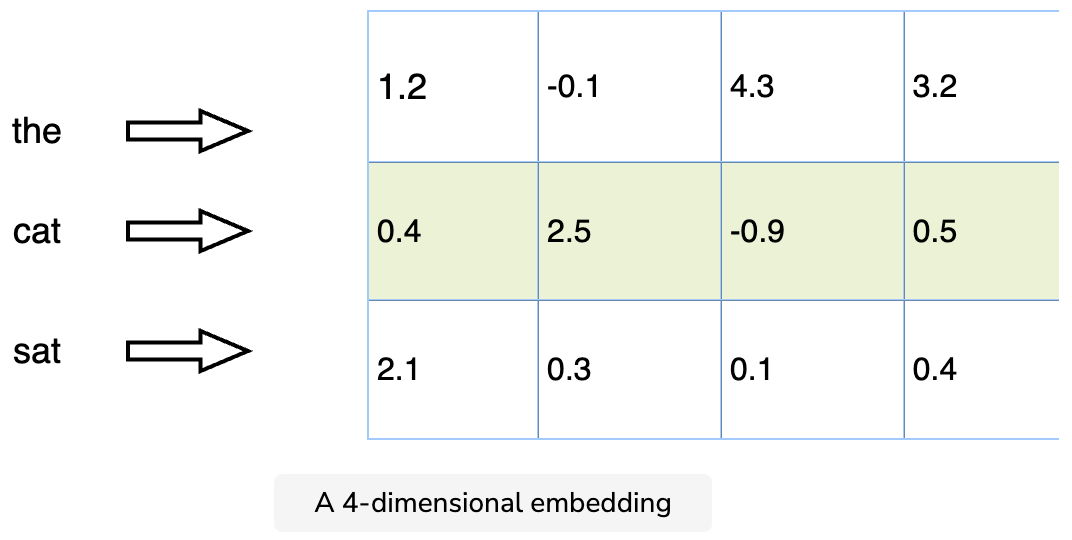
- As an example, each word can be represented as a d dimension vector, and we can train our supervised model. We then use the output of one of the fully connected layers of the neural network model as embeddings on the input object. For example, cat embedding can be represented as a [1.2, -0.1, 4.3, 3.2] vector.
How to generate/learn embedding vector?
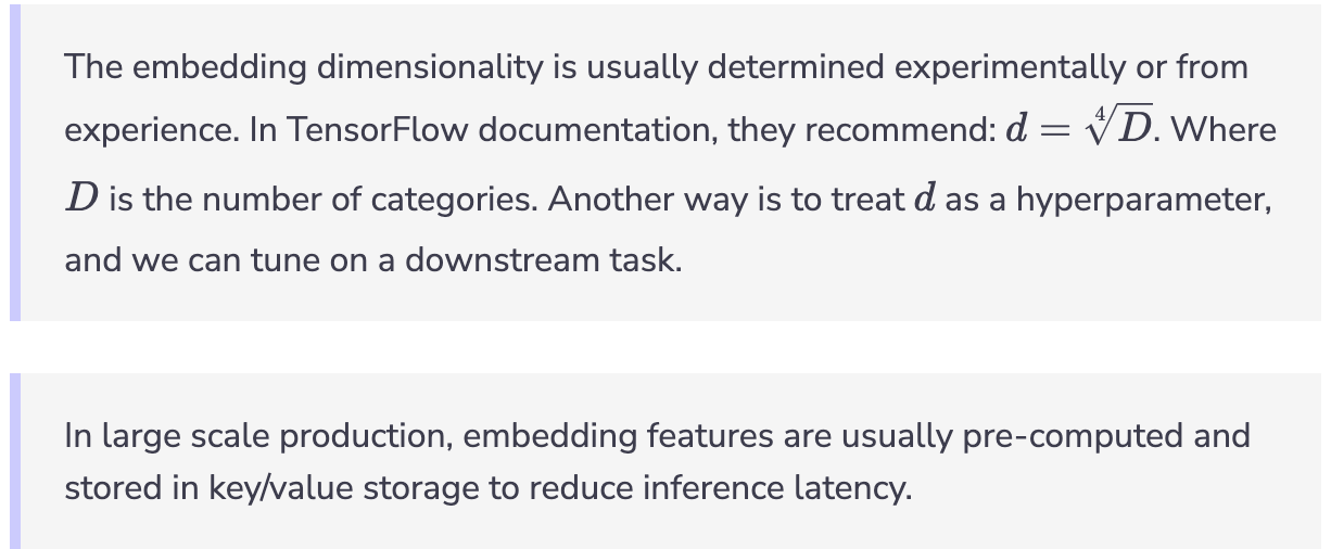
- For popular deep learning frameworks like TensorFlow, you need to define the dimension of embedding and network architecture. Once defined, the network can learn embedding automatically. For example:
# Embed a 1,000 word vocabulary into 5
dimensions.
embedding_layer =
tf.keras.layers.Embedding(1000, 5)
Embedding in tech companies
- This technique is commonly applied at many tech companies.
- Twitter uses Embedding for UserIDs and cases like recommendations, nearest neighbor searches, and transfer learning.
- Doordash uses Store Embedding (store2vec) to personalize the store feed. Similar to word2vec, each store is one word and each sentence is one user session. Then, to generate vectors for a consumer, we sum the vectors for each store they ordered from in the past 6 months or a total of 100 orders. Then, the distance between a store and a consumer is determined by taking the cosine distance between the store’s vector and the consumer’s vector.
- Similarly, Instagram uses account embedding to recommend relevant content (photos, videos, and Stories) to users.
Numeric features
- Normalization
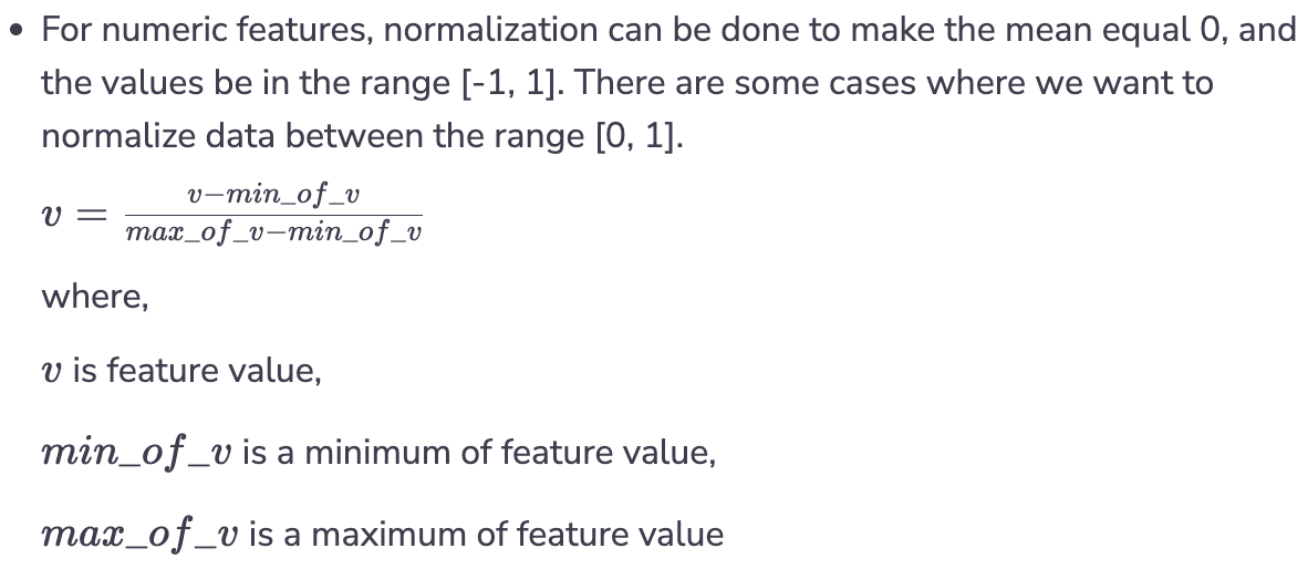
- For numeric features, normalization can be done to make the mean equal 0, and the values be in the range [-1, 1]. There are some cases where we want to normalize data between the range [0, 1].
- In practice, normalization can cause an issue as the values of min and max are usually outliers. One possible solution is “clipping”, where we choose a “reasonable” value for min and max.
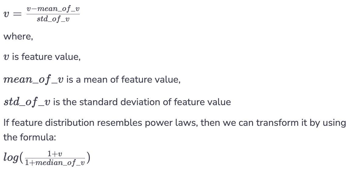
- Standardization
- If features distribution resembles a normal distribution, then we can apply a standardized transformation.
Training Pipeline
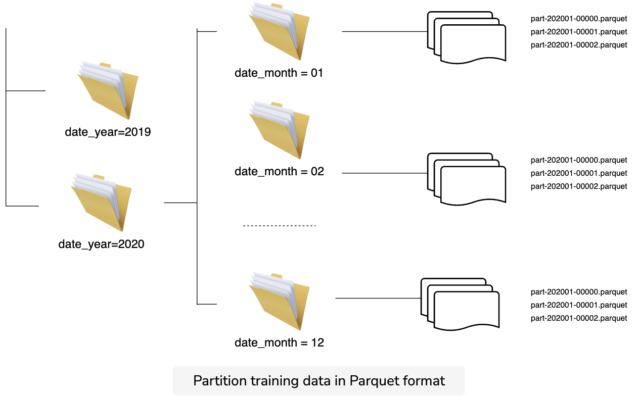
- A training pipeline needs to handle a large volume of data with low costs. One common solution is to store data in a column-oriented format like Parquet or ORC. These data formats enable high throughput for ML and analytics use cases. In other use cases, the tfrecord data format is widely used in the TensorFlow ecosystem.
Data partitioning
- Parquet and ORC files usually get partitioned by time for efficiency as we can avoid scanning through the whole dataset. In this example, we partition data by year then by month. In practice, most common services on AWS, RedShift, and Athena support Parquet and ORC. In comparison to other formats like csv, Parquet can speed up the query times to be 30x faster, save 99% of the cost, and reduce the data that is scanned by 99%.
Handle imbalance class distribution
- In ML use cases like Fraud Detection, Click Prediction, or Spam Detection, it’s common to have imbalance labels. There are few strategies to handle them, i.e, you can use any of these strategies depend on your use case.
- Use class weights in loss function: For example, in a spam detection problem where non-spam data has 95% data compare to other spam data which has only 5%. We want to penalize more in the non-spam class. In this case, we can modify the entropy loss function using weight.
//w0 is weight for class 0,
w1 is weight for class 1
loss_function = -w0 *
ylog(p) - w1*(1-y)*log(1-p)
- Use naive resampling: Resample the non-spam class at a certain rate to reduce the imbalance in the training set. It’s important to have validation data and test data intact (no resampling).
- Use synthetic resampling: The Synthetic Minority Oversampling Technique (SMOTE) consists of synthesizing elements for the minority class, based on those that already exist.
- It works by randomly picking a point from the minority class and computing the k-nearest neighbors for that point. The synthetic points are added between the chosen point and its neighbors. For practical reasons, SMOTE is not as widely used as other methods.
Choose the right loss function
- It depends on the use case when deciding which loss function to use. For binary classification, the most popular is cross-entropy. In the Click Through Rate (CTR) prediction, Facebook uses Normalized Cross Entropy loss (a.k.a. logloss) to make the loss less sensitive to the background conversion rate.
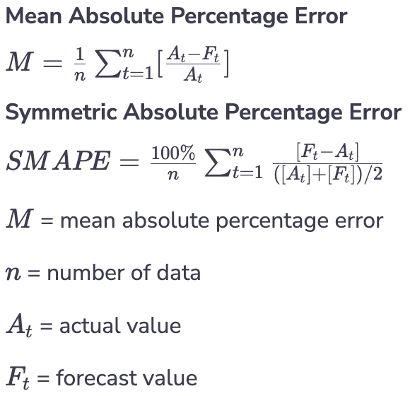
- In a forecast problem, the most common metrics are the Mean Absolute Percentage Error (MAPE) and the Symmetric Absolute Percentage Error (SMAPE). For MAPE, you need to pay attention to whether or not your target value is skew, i.e., either too big or too small. On the other hand, SMAPE is not symmetric, as it treats under-forecast and over-forecast differently.
- Other companies also use Machine Learning and Deep Learning for forecast problems. For example, Uber uses many different algorithms like Recurrent Neural Networks(RNNs), Gradient Boosting Trees, and Support Vector Regressors for various problems.
- Some of the problems include Marketplace forecasting, Hardware capacity planning, and Marketing.
- For the regression problem, DoorDash used Quantile Loss to forecast Food Delivery demand.
- The Quantile Loss is given by:
Retraining requirements
- Retraining is a requirement in many tech companies. In practice, the data distribution is a non-stationary process, so the model does not perform well without retraining.
- In AdTech and recommendation/personalization use cases, it’s important to retrain models to capture changes in user’s behavior and trending topics. So, machine learning engineers need to make the training pipeline run fast and scale well with big data. When you design such a system, you need to balance between model complexity and training time.
- A common design pattern is to use a scheduler to retrain models on a regular basis, usually many times per day.
Inference
- Inference is the process of using a trained machine learning model to make a prediction. Below are some of the techniques to scale inference in the production environment.
- Imbalance workload
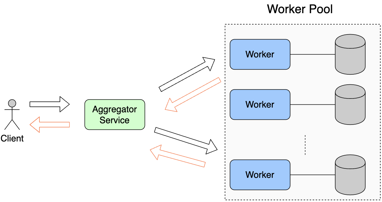
- During inference, one common pattern is to split workloads onto multiple inference servers. We use similar architecture in Load Balancers. It is also sometimes called an Aggregator Service.
- The image below shows Clients (upstream process) send requests to the Aggregator Service. If the workload is too high, the Aggregator Service splits the workload and sends it to workers in the Worker pool. Aggregator Service can pick workers through one of the following ways:
a) Work load
b) Round Robin
c) Request parameter
Wait for response from workers.
Forward response to client.
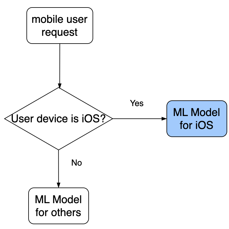
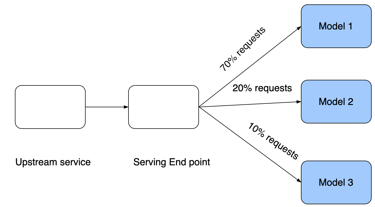
Serving logics and multiple models
- For any business-driven system, it’s important to be able to change logic in serving models. For example, in an Ad Prediction system, depending on the type of ad candidates, we will route to a different model to get a score.
Non-stationary problem
- In an online setting, data is always changing. Therefore, the data distribution shift is common. So, keeping the models fresh is crucial to achieving sustained performance. Based on how frequently the model performance degrades, we can then decide how often models need to update/retrain. One common algorithm that can be used is the Bayesian Logistic Regression.
Exploration vs. exploitation: Thompson Sampling
In an Ad Click prediction use case, it’s beneficial to allow some exploration when recommending new ads. However, if there are too few ad conversions, it can reduce company revenue. This is a well-known exploration-exploitation trade-off. One common technique is Thompson Sampling where at a time, we need to decide which action to take based on the reward.
Metrics evaluation
- In practice, it’s common that the model performs well during offline evaluation but does not perform well when in production. Therefore, it is important to measure model performance in both on and offline environments.
Offline metrics
During offline training and evaluating, we use metrics like logloss, MAE, and R2 to measure the goodness of fit. Once the model shows improvement, the next step would be to move to the staging/sandbox environment to test for a small percentage of real traffic.
Online metrics
- During the staging phase, we measure certain metrics, such as Lift in revenue or click through rate, to evaluate how well the model recommends relevant content to users. Consequently, we evaluate the impact on business metrics. If the observed revenue-related metrics show consistent improvement, then it is safe to gradually expose the model to a larger percentage of real traffic. Finally, when we have enough evidence that new models have improved revenue metrics, we can replace the current production models with new models. For further reading, explore how Sage Maker enables A/B testing or LinkedIn A/B testing.
- This diagram shows one way to allocate traffic to different models in production. In reality, there will be few a dozen models, each getting real traffic to serve online requests. This is one way to verify whether or not a model actually generates lift in the production environment.
Input Pipeline
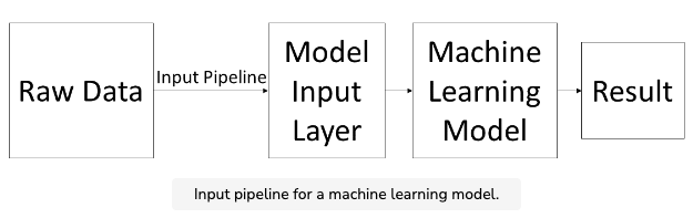
- Machine learning models are almost always trained on extremely large datasets. Depending on the application, a training dataset can have hundreds of thousands, or even millions, of training examples. The sheer size of these datasets makes it incredibly important to store the data in an efficient manner.
- The process in which data is loaded from files and fed into a machine learning model is known as the input pipeline. Since the input pipeline handles a large amount of data for machine learning projects, we need it to be as efficient as possible.
- A flexible and efficient format for storing large amounts of data is Google’s protocol buffer. The protocol buffer is similar to JSON and XML (another feature-based data format), but uses less space and is faster to process. When used with TensorFlow, protocol buffers make the input pipeline for large datasets much more streamlined.
Loading data
- One of the main reasons why protocol buffers work so well with TensorFlow is the ease with which they can be loaded as input into a machine learning model. Since TensorFlow is also a Google-developed product, the TensorFlow API contains functions that make it simple to quickly load data from a protocol buffer. This is why most of the official TensorFlow open-source models use protocol buffers for storing and loading data.
- In particular, the tf.data API provides us with all the tools necessary to create an efficient input pipeline. While it works very well with protocol buffers (which are used to store feature-based data), it can also be used effectively with NumPy data. In the following chapters, you’ll create input pipelines from both protocol buffers and NumPy data.
Feature Stores
- In machine learning, features and labels are fundamental components used to train and build predictive models. The relationship between features and labels is analogous to that of independent and dependent variables in a regression equation.
- In the context of machine learning, features refer to the independent variables or attributes that are used to make predictions or classify data. These features can be represented as columns in a table, where each column contains a specific attribute or characteristic of the data. For example, if we are building a model to predict housing prices, features could include attributes like the number of bedrooms, square footage, location, and so on. Features provide the necessary information for the model to make predictions or classify data based on patterns and relationships it learns from the training data.
- On the other hand, labels, also known as the dependent variable or target variable, represent the variable we are trying to predict or classify. In a regression equation, labels are the values that correspond to the dependent variable. In a table, the label typically corresponds to a specific column that we aim to predict based on the other columns (features) in the dataset. In the housing price prediction example, the label would be the actual sale price of a house.
- During the training phase, the model learns the relationships between the features and labels by analyzing the patterns and variations in the data. The model adjusts its internal parameters based on the provided features and corresponding labels, aiming to minimize the difference between its predicted values and the actual labels. Once trained, the model can then use the learned patterns to make predictions or classifications on new, unseen data.
- It’s worth noting that in some cases, certain columns in the dataset, such as unique identifiers or irrelevant attributes, are not useful for prediction purposes and are therefore dropped from the set of features.
- Features and labels are vital components in machine learning, enabling the model to learn and generalize patterns from the provided data, and make predictions or classifications based on those patterns.
- “What is a feature store? Well, it depends on who you ask. Some articles define it simply as “the central place to store curated features”. Others say it helps you “build features once; plug them anywhere” or “deploy models 100x faster”. There’s a wide range of definitions and I think it’s because what a feature store is depends on what you need.” (source)
Access
- In the context of building machine learning models, access to feature information and data is crucial for reducing duplication, encouraging reusability, and promoting efficient collaboration among teams. When access to feature information is low, organizations often encounter several challenges, including the duplication of efforts and resources, inconsistent results, and slower development processes for data science and machine learning teams.
- To address these challenges, companies like GoJek and Uber have developed feature stores that act as centralized platforms for managing and sharing features. These feature stores serve as interfaces between data engineers, scientists, and machine learning practitioners, allowing them to contribute, discover, and reuse features across different projects and teams.
- For example, GoJek’s Feast and Uber’s Palette feature stores enable data engineers and scientists to create and contribute features to a shared repository. ML practitioners can then consume these pre-built features from the store, eliminating the need to create the same features multiple times. This approach reduces duplication of effort, promotes consistency in machine learning outcomes, and accelerates the overall ML process.
- In addition to reducing duplication and encouraging reusability, feature stores also play a role in data discoverability. By making features easily findable and accessible, practitioners can quickly identify and utilize relevant features for their models. While not extensively discussed in the context of feature stores, data discoverability in feature stores is likely similar to the concepts discussed in open-sourced data discovery platforms.
- Feature stores serve as more than just repositories for features. They provide a convenient and efficient way for teams to collaborate, share, and reuse feature information, ultimately improving productivity and accelerating the development of machine learning models.
- SageMaker can facilitate the creation and management of feature stores for machine learning applications. SageMaker provides several features and services that can be leveraged to implement a feature store functionality.
- Amazon Athena is an interactive query service that allows you to analyze data directly in Amazon S3 using standard SQL queries. It can be used to query and explore your data stored in S3, including feature datasets. By defining appropriate schemas and partitions, you can create tables in Athena that represent your feature datasets.
- Once you have created the tables in Athena, you can leverage the querying capabilities to search and discover relevant features. You can run SQL queries to filter, aggregate, and analyze your feature data, allowing you to gain insights into the available features and their characteristics.
- With SageMaker, you can integrate Athena as a data source for your machine learning workflows. You can write queries in Athena to extract the required features and then use SageMaker for data preprocessing, model training, and deployment.
- While SageMaker itself does not provide native feature discoverability features, the combination of SageMaker and Athena enables you to leverage the querying capabilities of Athena to explore and discover features stored in your data lake or S3.
- By using SageMaker and Athena together, you can improve the discoverability of features, perform ad-hoc analysis on your feature datasets, and incorporate the discovered features into your machine learning pipelines.
Serving
- To address the challenge of serving features in real-time environments, Monzo Bank implemented a solution by automating the synchronization of features from their analytics store (BigQuery) to their production store (Cassandra).
- The process starts by adding tags to SQL queries that create feature tables within the analytics stack. These feature tables are updated at regular intervals, such as daily or hourly, ensuring that the features reflect the latest data.
- Next, a feature store Go service checks the schema of these feature tables, verifying that all the required columns, such as subject_type and subject_id, are present. This step ensures data consistency and completeness before serving the features.
- Finally, a cron job periodically checks for updated feature tables and synchronizes them from BigQuery to Cassandra. To facilitate the synchronization, a staging area in Google Cloud Storage is used as an intermediate step.
- By automating this synchronization process, Monzo Bank ensures that the features used during model training in their analytics stack are made available in their production environment for real-time serving. This allows them to maintain consistency between offline training and online serving and enables them to leverage the trained models with the required features in a high-throughput and low-latency manner.
Uber’s feature store
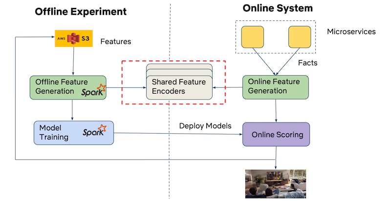
- The image below (source) show on the left how creating batch and on the right, real-time features and synchronization between stores happens.
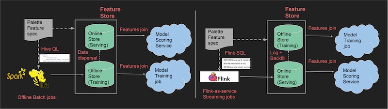
- Uber’s feature store, Palette, follows a dual-store approach to handle offline and real-time serving of features. The offline store, implemented using Hive, stores feature snapshots and primarily serves the training jobs. On the other hand, the online store utilizes Cassandra to serve the same features in real-time.
- In the Palette architecture, features that are not readily available in Cassandra are generated in real-time using Apache Flink, a stream processing framework. These generated features are then saved to Cassandra, ensuring that they are accessible for real-time serving.
- To maintain consistency and synchronization between the offline and online stores, data movement is orchestrated. When new features are added to Hive, they are automatically copied to Cassandra to make them available for real-time serving. Similarly, any real-time features added to Cassandra are extracted, transformed, and loaded (ETL-ed) to Hive, ensuring that they are accessible for batch processing and offline training jobs.
- This synchronization process ensures that the feature data is consistent and up-to-date across both the offline and online stores, enabling seamless transitions between training models offline and serving them in real-time using the appropriate set of features.
DoorDash feature store
- DoorDash faced significant technical requirements when building their Gigascale feature store to address their serving needs. These requirements included:
- Storing billions of records: Due to the large number of entities such as users, merchants, and food items, DoorDash needed a feature store capable of handling billions of feature-value pairs. This required a persistent and scalable storage solution.
- Handling millions of queries per second (QPS): The feature store was accessed by multiple use cases, including store ranking, which relied on dozens of features and made over 1 million predictions per second. Considering DoorDash’s production models, the feature store had to handle more than 10 million QPS.
- Daily refreshes with fast batch writes: Most of the features in the store required daily updates, while real-time features, such as each store’s delivery time over a 20-minute moving average, needed uniform updates throughout the day. This required efficient batch write capabilities to refresh the feature values.
- To build their Gigascale feature store, DoorDash conducted benchmarking tests on various key-value stores, including Redis, Cassandra, CockroachDB, ScyllaDB, and YugabyteDB. After evaluating their performance, DoorDash chose Redis as the storage solution for their feature store. They also optimized Redis to meet their specific requirements, as documented in their detailed write-up.
- By carefully selecting and optimizing Redis, DoorDash was able to build a feature store that could handle their massive scale, provide high throughput for queries, and efficiently refresh feature values on a daily basis.
Alibaba feature store
- In the case of Alibaba, they adopt a different approach for serving real-time recommendations by computing features in real-time. They have implemented the Alibaba Basic Feature Server, which performs real-time computation of statistical features based on user interactions such as clicks, likes, and purchases. These computed features are then utilized for candidate generation in their recommendation system.
- By computing features in real-time, Alibaba can capture the most up-to-date user behavior and incorporate it into the recommendation process. This approach enables them to provide personalized and relevant recommendations to their users based on their recent interactions. Real-time computation of features allows for dynamic and responsive recommendations that adapt to the changing user preferences and behaviors.
- The use of real-time features in candidate generation enhances the accuracy and timeliness of the recommendations provided by Alibaba. It enables them to consider the most relevant and recent user signals, improving the overall effectiveness of their recommendation system.
- It’s worth noting that this approach aligns with the concept of real-time recommendations discussed earlier, where time-sensitive missions and context-dependent recommendations benefit from the availability of up-to-date features. By computing features in real-time, Alibaba ensures that their recommendation system can adapt to the immediate needs and preferences of their users, enhancing the user experience and increasing the effectiveness of their recommendations.
Integrity
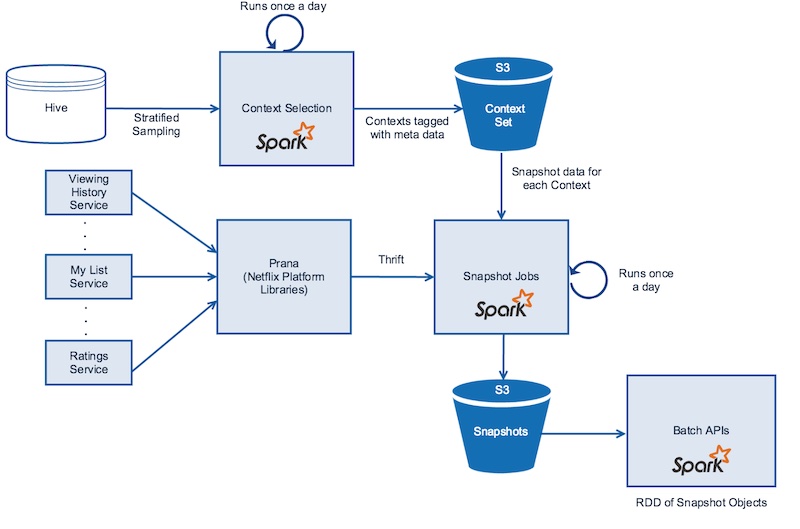
- The image below (source) creates a snapshots from offline stores and online micro services
- To ensure the integrity of offline and online features, companies like Netflix and GoJek have implemented strategies to address two main pain points: creating point-in-time accurate features and maintaining consistency between features used in training and serving.
- Netflix has developed a distributed time-travel system to create accurate snapshots of both offline and online data. These snapshots capture various contextual information such as member type, device, and time of day. However, creating snapshots for every context can be resource-intensive, so Netflix employs stratified sampling on attributes like viewing patterns, device type, time spent on device, and region. This sampling approach provides a representative distribution of data for training and validating their models. Spark is used for sampling, and the resulting snapshots are stored in S3.
- Similarly, Netflix takes snapshots of online data from their microservices, which provide data such as viewing history, personalized viewing queues, and predicted ratings. Spark parallelizes the calls to retrieve data from these microservices using a component called Prana. The resulting snapshots are also stored in S3, typically using the Parquet format.
- To address the issue of train-serve skew, GoJek has adopted Apache Beam as their data processing pipeline. This allows them to ingest data from various sources, including batch and streaming sources like BigQuery and Kafka. The data is then processed and stored in offline and online stores such as BigQuery and Redis, respectively. By using a unified API, GoJek minimizes the need to rewrite feature pipelines for the serving environment, reducing the risk of introducing inconsistencies between training and serving. This approach helps ensure that the models perform optimally when deployed online.
- By implementing these strategies, companies like Netflix and GoJek strive to maintain the integrity of their features throughout the machine learning lifecycle. They focus on creating accurate snapshots of data and ensuring consistency between training and serving environments, ultimately improving the performance and reliability of their machine learning models in real-world production scenarios.
Data flywheel
- The concept of the “Data Flywheel” refers to a pattern where continuous data collection leads to model improvement, which in turn enhances the user experience. This positive feedback loop generates more usage, resulting in the accumulation of additional data that can further improve the models. The Data Flywheel is considered a potent source of long-term competitive advantage, as it relies on the continuous refinement of models based on accumulating data.
- One of the significant advantages of the Data Flywheel is that it can create a sustainable competitive advantage, as the collected data becomes a valuable asset. While model architectures and system designs can be replicated or imitated, the accumulated data remains unique and difficult to replicate. It forms the foundation for building more accurate and effective models, driving better user experiences.
- However, there are potential drawbacks to consider. One challenge is the perpetuation of biases within the data. For example, in recommendation systems, there is a risk of popularity bias, where popular items tend to receive more exposure and recommendations, leading to a reinforcing loop. Data augmentation techniques can help alleviate this issue by introducing diversity and mitigating biases.
- Amazon and Netflix are prime examples of companies that leverage the Data Flywheel pattern. Both platforms collect extensive data on user behavior, such as searches, clicks, ratings, and watch time. This data is used to train recommendation systems that learn from individual preferences and deliver personalized recommendations. As users engage more with the platform and generate additional data, the recommendations become more accurate and relevant, leading to increased user satisfaction and usage.
- Tesla’s Autopilot system is another example of the Data Flywheel in action. Tesla collects driving images and videos from its vehicles, which serve as a valuable data source for improving their autonomous driving models. By analyzing this data, Tesla can identify errors, find similar instances (nearest neighbors), and label them. These newly labeled data points are then used to retrain the models, which are subsequently deployed to Tesla vehicles. As the vehicles continue to gather more driving data, the cycle repeats, continually refining and enhancing the autonomous driving capabilities.
- Data Flywheel pattern revolves around the continuous collection of data, which fuels model improvement and enhances the user experience. It has been successfully employed by companies like Amazon, Netflix, and Tesla to create competitive advantages and deliver more personalized and effective services.
Evaluate before deploy via Validation set
- The “Evaluate before Deploy” pattern emphasizes the importance of thoroughly evaluating model and system performance before integrating them into production. This practice aims to ensure safety, reliability, and the ability to meet user experience and business objectives. Similar to testing software builds before deployment, evaluating models before deploying them is crucial.
- The main advantage of this pattern is that it reduces the risk of deploying models with poor performance, biased predictions, or other issues that could have a negative impact on the user experience or business outcomes. By conducting thorough evaluations, organizations can make informed decisions about whether a model is ready for deployment.
- To implement this pattern, one common approach is to have a validation hold-out during the (re)training of models. Typically, the validation set should be split based on time, considering the temporal nature of most production systems. Random splits or cross-validation can lead to overly optimistic evaluation metrics if future data leaks into the training set.
- For example, in the context of recommendation systems, the last period of data (such as the last day or hour) can be held out as a validation set. The models can be refreshed based on new data and evaluated on the validation set using standard metrics like hit@k (the number of relevant items in the top-k recommendations), NDCG (Normalized Discounted Cumulative Gain), and others. It’s also common to compare the performance against a naive baseline, such as a popularity-based sorting approach, to assess the improvement achieved by the model.
- If the refreshed model fails to meet the desired evaluation metrics or performs worse than the baseline, it is recommended to halt the deployment pipeline and refrain from releasing the model into production. It’s better to have a stale model in production than one that behaves poorly or has subpar performance.
- “Evaluate before Deploy” pattern advocates for thorough evaluation of model and system performance before integrating them into production. This practice helps mitigate risks and ensures that deployed models meet the desired performance standards, enhancing user experience and achieving business objectives.